Censoring occurs when values of a variable within a certain range are unobserved, but it is known that the variable falls within this range. This differs from truncation, where values of a variable within a certain range are unobserved and it is unknown when the variable falls within this range. Both phenomena represent a loss of information, but the loss is less with censoring than with truncation. The two are sometimes confused in the literature; some examples are given in Leopold Simar and Paul Wilson (2007). George Maddala (1983) and Takeshi Amemiya (1984) list a number of empirical applications where censoring occurs.
In models of duration, right-censoring often occurs, but left-censoring can also occur. For example, if agents are observed in some state (e.g., unemployment, in the case of individuals, or solvency, in the case of firms) until either they are observed to exit the state or until the period of observation ends, then some agents may still be in the given state at the end of the observation window. Observations on these agents will be right-censored. Similarly, at the beginning of the study, some (perhaps all) agents are observed to be already in the state of interest; for any agents whose time of entry into the state is unknown, their duration in the given state is left-censored (and perhaps also right-censored).
To illustrate censoring in a regression context, suppose
where E(ei) = 0. If Y. is censored, then one must estimate the model
after replacing Y. in (1) with Y., which necessarily results in a new error term in (2). Unless the censoring occurs in the extreme tails of the distribution of Y, ordinary least squares (OLS) estimation of the coefficients in (2) will yield biased and inconsistent estimates since OLS does not account for the censoring.
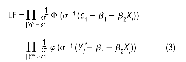
Censored regression models are typically estimated by the maximum likelihood method. If the errors in model (1) are assumed normally distributed with mean 0 and variance a2, then in the case of left-censoring at c1 the likelihood function is given by
where ^ and # denote the standard normal density and distribution functions, respectively. This model was first proposed by James Tobin (1958), and is sometimes called the tobit model. The first product in (3) gives, for each observed value Y. equal to cx, the probability of obtaining a draw Y. from F(y) less than c1.
The models presented above potentially suffer from several problems. Heteroskedasticity in the error terms can lead to inconsistent estimation. D. Petersen and Donald Waldman (1981) proposed modifications of the tobit-type models involving specification of particular models for the error variances. John Cragg (1971) proposed a generalized version of the tobit model that allows the probability of censoring to be independent of the regression model for the uncensored data. Perhaps the most vexing problem is the requirement of a distributional assumption for the errors in (2). It is straightforward to assume distributions other than the normal distribution and then work out the resulting likelihood functions, but rather more difficult to avoid such assumptions altogether by using semi- or nonparametric methods. Adrian Pagan and Aman Ullah (1999) discuss several proposals, but these involve significant increases in computational burden or data requirements.


