Viewing and modeling transformations are inextricably related in OpenGL and are in fact combined into a single modelview matrix. (See "A Simple Example: Drawing a Cube" on page 109.) One of the toughest problems newcomers to computer graphics face is understanding the effects of combined three-dimensional transformations. As you’ve already seen, there are alternative ways to think about transformations—do you want to move the camera in one direction or move the object in the opposite direction? Each way of thinking about transformations has advantages and disadvantages, but in some cases one way more naturally matches the effect of the intended transformation. If you can find a natural approach for your particular application, it’s easier to visualize the necessary transformations and then write the corresponding code to specify the matrix manipulations. The first part of this section discusses how to think about transformations; later, specific commands are presented. For now, we use only the matrix-manip-ulation commands you’ve already seen. Finally, keep in mind that you must call glMatrixMode() with GL_MODELVIEW as its argument prior to performing modeling or viewing transformations.
Thinking about Transformations
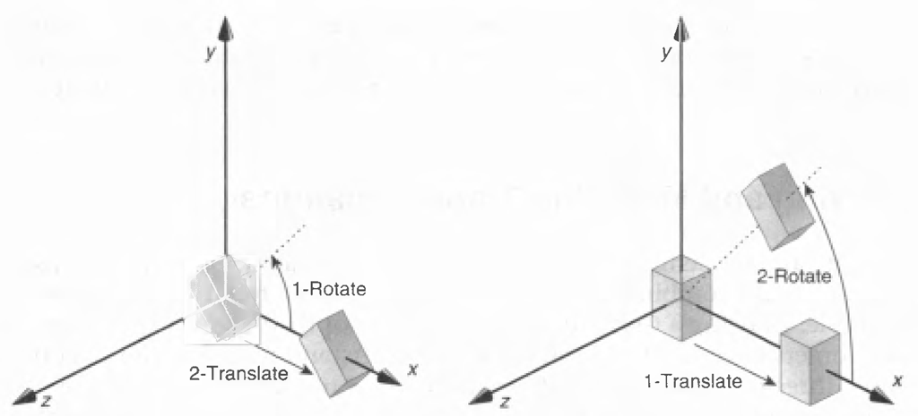
Let’s start with a simple case of two transformations: a 45-degree counterclockwise rotation about the origin around the z-axis and a translation down the x-axis. Suppose that the object you’re drawing is small compared with the translation (so that you can see the effect of the translation) and that it’s originally located at the origin. If you rotate the object first and then translate it, the rotated object appears on the x-axis. If you translate it down the A>axis first, however, and then rotate about the origin, the obiect is on the line y = x, as shown in Figure 3-4. In general, the order of transformations is critical. If you do transformation A and then transformation B, you almost always get something different than if you do them in the opposite order.
Figure 3-4 Rotating First or Translating First
Now let’s talk about the order in which you specify a series of transformations. All viewing and modeling transformations are represented as 4 χ 4 matrices. Each successive glMultMatrix*() or transformation command multiplies a new 4×4 matrix M by the current modelview matrix C to yield CM. Finally, vertices v are multiplied by the current modelview matrix. This process means that the last transformation command called in your pro- . gram is actually the first one applied to the vertices: CMv. Thus, one way of looking at it is to say that you have to specify the matrices in the reverse order. Like many other things, however, once you’ve gotten used to thinking about this correctly, backward will seem like forward.
Consider the following code sequence, which draws a single point using three transformations:
With this code, the modelview matrix successively contains I, N, NM, and finally NML, where I represents the identity matrix. The transformed vertex is NMLv. Thus, the vertex transformation is N(M(Lv))—that is, v is multiplied first by L, the resulting Lv is multiplied by M, and the resulting MLv is multiplied by N. Notice that the transformations to vertex v effectively occur in the opposite order than they were specified. (Actually, only a single multiplication of a vertex by the modelview matrix occurs; in this example, the N, M, and L matrices are already multiplied into a single matrix before it’s applied to v.)
Grand, Fixed Coordinate System
Thus, if you like to think in terms of a grand, fixed coordinate system—in which matrix multiplications affect the position, orientation, and scaling of your model—you have to think of the multiplications as occurring in the opposite order from how they appear in the code. Using the simple example shown on the left side of Figure 3-4 (a rotation about the origin and a translation along the x-axis), if you want the object to appear on the axis after the operations, the rotation must occur first, followed by the translation. To do this, you’ll need to reverse the order of operations, so the code looks something like this (where R is the rotation matrix and T is the translation matrix):
Moving a Local Coordinate System
Another way to view matrix multiplications is to forget about a grand, fixed coordinate system in which your model is transformed and instead imagine that a local coordinate system is tied to the object you’re drawing. All operations occur relative to this changing coordinate system. With this approach, the matrix multiplications now appear in the natural order in the code. (Regardless of which analogy you’re using, the code is the same, but how you think about it differs.) To see this in the translation-rotation example, begin by visualizing the object with a coordinate system tied to it. The translation operation moves the object and its coordinate system down the x-axis. Then, the rotation occurs about the (now-translated) origin, so the object rotates in place in its position on the axis.
This approach is what you should use for applications such as articulated robot arms, where there are joints at the shoulder, elbow, and wrist, and on each of the fingers. To figure out where the tips of the fingers go relative to the body, you’d like to start at the shoulder, go down to the wrist, and so on, applying the appropriate rotations and translations at each joint. Thinking about it in reverse would be far more confusing.
This second approach can be problematic, however, in cases where scaling occurs, and especially so when the scaling is nonuniform (scaling different amounts along the different axes). After uniform scaling, translations move a vertex by a multiple of what they did before, as the coordinate system is stretched. Non-uniform scaling mixed with rotations may make the axes of the local coordinate system nonperpendicular.
As mentioned earlier, you normally issue viewing transformation commands in your program before any modeling transformations. In this way, a vertex in a model is first transformed into the desired orientation and then transformed by the viewing operation. Since the matrix multiplications must be specified in reverse order, the viewing commands need to come first. Note, however, that you don’t need to specify either viewing or modeling transformations if you’re satisfied with the default conditions. If there’s no viewing transformation, the "camera" is left in the default position at the origin, pointing toward the negative z-axis; if there’s no modeling transformation, the model isn’t moved, and it retains its specified position, orientation, and size.
Since the commands for performing modeling transformations can be used to perform viewing transformations, modeling transformations are discussed first, even if viewing transformations are actually issued first. This order for discussion also matches the way many programmers think when planning their code. Often, they write all the code necessary to compose the scene, which involves transformations to position and orient objects correctly relative to each other. Next, they decide where they want the viewpoint to be relative to the scene they’ve composed, and then they write the viewing transformations accordingly.
Modeling Transformations
The three OpenGL routines for modeling transformations are glTrans!ate*(), glRotate*(), and glScale*(). As you might suspect, these routines transform an object (or coordinate system, if you’re thinking of it in that way) by moving, rotating, stretching, shrinking, or reflecting it. All three commands are equivalent to producing an appropriate translation, rotation, or scaling matrix, and then calling glMultMatrix*() with that matrix as the argument. However, using these three routines might be faster than using glMultMatrix*(). OpenGL automatically computes the matrices for you.
In the command summaries that follow, each matrix multiplication is described in terms of what it does to the vertices of a geometric object using the fixed coordinate system approach, and in terms of what it does to the local coordinate system that’s attached to an object.
Translate
void glTranslate{fd}(7TP£ x, TYPE y, TYPE /);
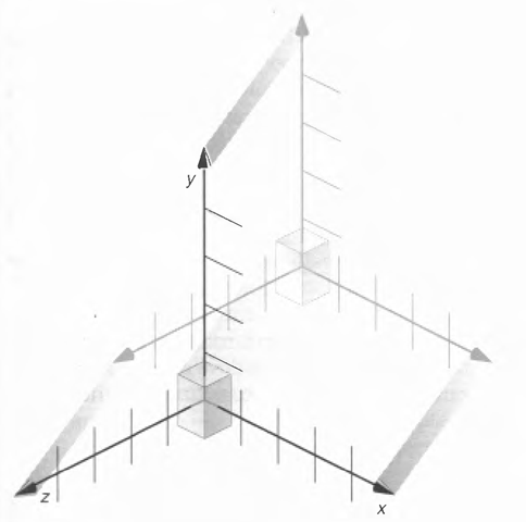
Multiplies the current matrix by a matrix that moves (translate^ an object by the given x-, y-, and z-values (or moves the local coordinate system by the same amounts).
Figure 3-5 shows the effect of glTranslate*().
Figure 3-5 Translating an Object
Note that using (0.0, 0.0, 0.0) as the argument for glTranslate*() is the identity operation—that is, it has no effect on an object or its local coordinate system.
Rotate
void glRotate’fd}(TYPE angle, TYPE x, TYPE y, TYPE z);
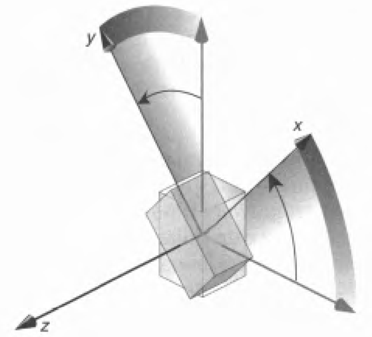
Multiplies the current matrix by a matrix that rotates an object (or the local coordinate system) in a counterclockwise direction about the ray from the origin through the point (x, y, z). The angle parameter specifies the angle of rotation in degrees.
The effect of glRotatef(45.0, 0.0, 0.0, 1.0), which is a rotation of 45 degrees about the z-axis, is shown in Figure 3-6.
Figure 3-6 Rotating an Object
Note that an object that lies farther from the axis of rotation is more dramatically rotated (has a larger orbit) than an object drawn near the axis. Also, if the angle argument is zero, the glRotate*() command has no effect.
Scale
void glScalejfd}{TYPE x, TYPE y, TYPE z);____
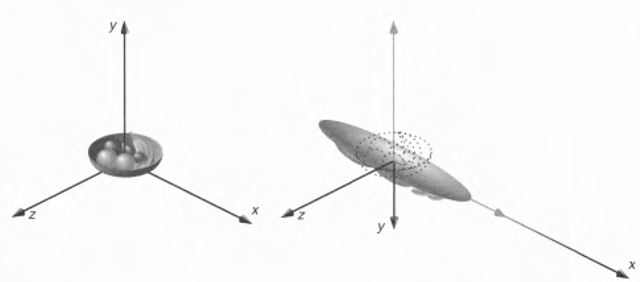
Multiplies the current matrix by a matrix that stretches, shrinks, or reflects an object along the axes. Each x-, y-. and z-coordinate of every point in the object is multiplied by the corresponding argumeni x, y, or z. With the local coordinate system approach, the local coordinate axes are stretched, shrunk, or reflected by the x-, y-, and z-factors, and the associated object is transformed with them.
Figure 3-7 shows the effect of glScalef(2.0, -0.5, 1.0).
Figure 3-7 Scaling and Reflecting an Object
glScale*() is the only one of the three modeling transformations that changes the apparent size of an object: scaling with values greater than 1.0 stretches an object, and using values less than 1.0 shrinks it. Scaling with a -1.0 value reflects an object across an axis. The identity values for scaling are (1.0, 1.0, 1.0). In general, you should limit your use of glScale*() to those cases where it is necessary. Using glScale*() decreases the performance of lighting calculations, because the normal vectors have to be renormalized after transformation.
Note: A scale value of zero collapses all object coordinates along that axis to zero. It’s usually not a good idea to do this, because such an operation cannot be undone. Mathematically speaking, the matrix cannot be inverted, and inverse matrices are required for certain lighting operations.Sometimes collapsing coordinates does make sense; the calculation of shadows on a planar surface is one such application.In general, if a coordinate system is to be collapsed, the projection matrix should be used, rather than the modelview matrix.


