Fuzzy Logic (Microcontrollers)

7.6
This section, taken from the Motorola CPU 12 reference manual (Rev. 1), section 9, gives a general introduction to fuzzy logic concepts and illustrates an implementation of fuzzy logic programming. There are a number of fuzzy logic programming strategies; this discussion concentrates on the methods that use 6812 fuzzy logic instructions.
In general, fuzzy logic provides for set definitions that have fuzzy boundaries rather than the crisp boundaries of Boolean logic. A Boolean variable is either true or false, while in fuzzy logic, a linguistic variable has a value that is a degree of confidence between 0 and 1. A value can be “0.2 (or 20%) confident.” For a specific input value, one or more linguistic variables may be confident to some degree at the same time, and their sum need not be 1. As an input varies, one linguistic variable may become progressively less confident while another becomes progressively more confident.
Fuzzy logic membership junctions better emulate human concepts like “I got a B on the last quiz” than Boolean functions that are either absolutely true or absolutely false; that is, conditions are perceived to have gradual or fuzzy boundaries. Despite the term “fuzzy,” a specific set of input conditions always deterministically produces the same result, just as in conventional control systems. Fuzzy sets provide a means of using linguistic expressions like “I got a B” in rules that can then be evaluated with numerical precision and repeatability. We will see that fuzzy membership functions help solve certain types of complex problems that have eluded traditional methods, as we study how fuzzy logic could compute a student’s course grade from his or her quiz scores.
An application expert, without any microcontroller programming experience, can generate a knowledge base. In it, membership functions express an understanding of the system’s linguistic terms. And in it, ordinary language statement rules describe how a human expert would solve the problem. These are reduced to relatively simple data structures (the knowledge base) that reside in the microcontroller memory.

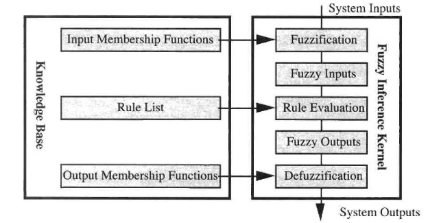
Figure 7.21. Fuzzy Logic Control System
A microcontroller-based fuzzy logic control system has a fuzzy inference kernel and a knowledge base. See Figure 7.21. The fuzzy inference kernel is executed periodically to determine system outputs based on current system inputs. The knowledge base contains membership functions and rules.
A programmer who does not know how the application system works can write a fuzzy inference kernel. One execution pass through the fuzzy inference kernel generates system output signals in response to current system input conditions. As in a conventional control system, the kernel is executed as often as needed to maintain control. If the kernel is executed too often, processor bandwidth and power are wasted;

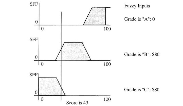
Figure 722. Membership Functions
but if too infrequently, the system gets too far out of control. The steps of this kernel are: fuzzification, rule evaluation, and defuzzification.
During fuzzification, the current system input values are compared against stored input membership functions, usually in a program loop structure, to determine the degree to which each linguistic variable of each system input is true. Three membership functions are indicated in Figure 7.22; these convert a student’s quiz test score to a letter grade. This is accomplished by finding the y-value for the current input value on a trapezoidal membership function for each label of each system input. If a student’s test score is 43, his or her membership in linguistic variable “Grade is A’* is zero, in linguistic variable “Grade is B” is $80 (50%). and in linguistic variable “Grade is C” is $80 (50%). Fuzzy logic avoids the agony of missing a “B” by a point or two.
In our example, system inputs are each quiz’s and homework assignment’s numeric grades. Linguistic variable values are the degree of confidence that the student has a particular grade associated with each letter grade. If there are two quizzes and one homework assignment, and each has three grades, then there are nine linguistic variables.
The end result of the fuzzification step is a collection of fuzzy linguistic variables reflecting the system. This is passed to the rule evaluation phase, which processes a list of rules from the knowledge base using current fuzzy input values to produce a list of fuzzy output linguistic variables. These fuzzy outputs are considered raw suggestions for what the system output should be in response to the current input conditions. The following is an example of a typical rule:
If you get an A on quiz 1, an A on quiz 2, and an A on homework assignments, then you should get an A+ for the course.
The left portion of the rule is a statement of input conditions, antecedents connected by a fuzzy AND operator, and the right portion of the rule is a statement of output actions called consequents.
In an automotive antiskid braking system, about 600 such rules are used to compute the brake pressure to be applied. Analogous to the Boolean sum-of-products, rule evaluation employs a fuzzy AND operator, used to connect antecedents within a rule, and a fuzzy OR operator, which is implied among all rules affecting a given consequent. Each rule is evaluated sequentially, but the rules as a group are treated as if they were all evaluated simultaneously. The AND operator corresponds to the mathematical minimum operation, and the fuzzy OR operation corresponds to the maximum operation. Before evaluating any rules, all fuzzy outputs are set to zero (meaning none are true). As each rule is evaluated, the minimum antecedent is taken to be the overall confidence of the rule result. If two rules affect the same fuzzy output, the rule that is most true governs the value in the fuzzy output, because the rules are connected by an implied fuzzy OR. There is also a fuzzy negate operator, which complements each bit.
Each antecedent expression consists of the name of a system input, followed by “is,” followed by a label name defined by a membership function in the knowledge base. Because “and” is the only operator allowed to connect antecedent expressions, there is no need to include these in the encoded rule. Each consequent expression consists of the name of a system output, followed by “is,” followed by a label name; for example:
If quiz 1 is A, quiz 2 is A, homework assignment is A, then course is A+.
Rules can be weighted. The confidence value for a rule is determined as usual by finding the smallest rule antecedent. Before applying this value to the consequents for the rule, the value is multiplied by a fraction from zero (rule disabled) to $FF (rule fully enabled). The resulting modified confidence value is then applied to the fuzzy outputs. Equation (19) illustrates that the output for a set of rules is the output Sj for each rule times a weight Fj, divided by the sum of the weights.
The rules can reflect nonlinear, but deterministic, relationships. For instance, if a student gets a B on the first quiz and an A on the second quiz, the instructor may decide that the course grade is A-, but if a student gets an A on the first quiz and a B on the second quiz, the instructor may decide that the course grade is B+. But if the student also did poorly in lab work, then the course grade might be B-, to give the student some incentive to get to work. That is, if quiz 1 is A, quiz 2 is B, and lab is not C, then course is B+, but if quiz 1 is A, quiz 2 is B, and lab is C, then course is B-. In the limit, if there are n input variables and each input variable is associated with m linguistic
* Fuzzification step:

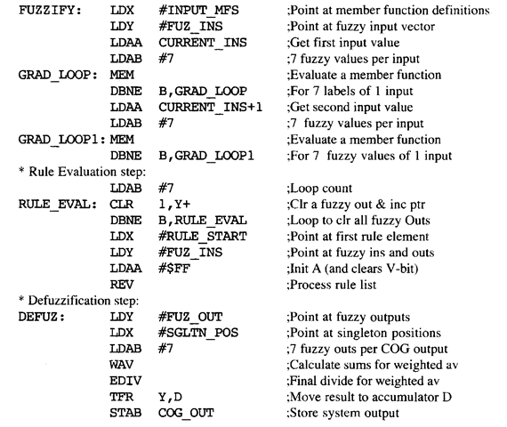
Figure 7.23. A Fuzzy Inference Kernel
variables, then there can be as many as nm rules to produce each output linguistic variable, one to cover each case. That would be unattractive, but heuristics are used to substantially reduce this number of rules using common sense.
But before the results can be applied, fuzzy outputs must be further processed, or defuzzified, to produce a single output value that represents the combined effect of all of the fuzzy outputs. In our example, a single output would be a numerical grade for the course. The end result of the rule evaluation step is a collection of suggested or “raw” fuzzy outputs. These values were obtained by plugging current conditions (fuzzy input values) into the system rules in the knowledge base. The raw results cannot be supplied directly to the system outputs because they may be ambiguous. For instance, one raw output can indicate that a grade should be B+ with a degree of confidence of 50% while, at the same time, another indicates that the grade should be C- with a degree of confidence of 25%. A simple “max defuzzification” technique, which outputs the maximum of all the degrees of confidence, ignores all other degrees of confidence, and gives inferior results. A better defuzzification step resolves multiple-degree ambiguities by combining the raw fuzzy outputs into a composite numerical output using singletons. The singleton for a linguistic variable is a single value assigned to the output variable if the rules produce this linguistic variable with a degree of confidence of 1, and all other linguistic variables have a degree of confidence of zero. For instance, the singleton for A+ might be 100, the singleton for A might be 95, that for A- might be 90, and so on. Singletons Sj are weighted by fuzzy output degrees of confidence Fj, for n such outputs, normalized to a degree of confidence of one, in the expression (19)

Figure 7.23 shows a 6812 fuzzy inference kernel. When the fuzzification step begins, a MEM instruction fuzzifies the inputs. The current value of the system input is in accumulator A, index register X points to the first membership function definition, and a index register Y points to the first fuzzy input. As each fuzzy input is calculated by executing a MEM instruction, the result is stored to the fuzzy input, and both X and Y are updated automatically to point to the locations associated with the next fuzzy input. For each system input, a DBNE instruction executes as many MEM instructions as a system input has fuzzy input linguistic variables. Thus MEM and DBNE handle one system input’s fuzzification. Repeated such program segments handle each system input.
Each trapezoidal membership function is defined by four 8-bit parameters, XI, X2, SI, and S2. XI is where the trapezoid’s left slope intercepts Y = 0, and X2 is where the trapezoid’s right slope intercepts Y = 0. SI is the trapezoid’s left slope (AY/AX), and S2 is the trapezoid’s right slope (-AY/AX), but a slope of 0 is defined as a vertical line.
More complicated membership functions can be evaluated by the TBL instruction, which interpolates arbitrary table functions. A 16-bit version of TBL, ETBL, permits handling 16-bit input variables and 16-bit degrees of confidence.
The rule evaluation step is likewise almost completely executed by the REV instruction. Before it is executed, fuzzy outputs are cleared, index register X points to a vector of the rules, Y points to the base address of fuzzy inputs and outputs, and accumulator A is set for maximum ($FF). Each antecedent expression is represented as an 8-bit relative offset from index register Y, to read an 8-bit fuzzy input. Antecedents are separated from consequents with reserved “offset” value $FE. Each consequent expression
is represented as an 8-bit relative offset from index register Y, to write an 8-bit fuzzy output. The consequents end with a reserved value $FE, if more rules must be evaluated, or $FF, after the last rule is evaluated. The condition code V signifies whether antecedents are being processed (V = 0) or consequents are being processed (V = 1).
Besides REV, the more complex REVW instruction allows each rule to have a separate weighting factor, and EMIND and EMAXD can be used to implement 16-bit rule evaluation.
The WAV instruction calculates the numerator and denominator sums for weighted average of the fuzzy outputs. Before executing WAV, accumulator B must be loaded with the number of iterations, index register Y must be pointed at the list of singleton positions in the knowledge base, and index register X must be pointed at the list of fuzzy outputs in RAM. If the system has more than one system output, the WAV instruction is executed once for each system output. The final divide is performed with a separate EDI V instruction placed immediately after the WAV instruction.
The EM ACS instruction can be used to evaluate 16-bit linguistic variables. A separate but simple program segment must calculate the sum of linguistic variables, which is automatically calculated by the WAV instruction.
The 6812 is currently the only microcontroller that has machine instructions that can be used to implement the complete fuzzy inference kernel. These machine instructions speed up execution of the kernel by a factor of about 10 over software evaluation that uses ordinary instructions. This feature makes the 6812 the microcontroller of choice for time-critical applications that use fuzzy logic.
In conclusion, fuzzy logic provides fuzzy rather than crisp boundaries. Linguistic variables indicate a degree of confidence. Combinations of variables are presumed to be true to the worst-case (minimum) degree of confidence, and alternatives are presumed to be true to the best-case (maximum) degree of confidence. Final values are weighted sums of typical values, using degrees of confidence as weights. Such fuzzy logic systems are currently being applied to automotive control and other rather complex control systems.