1.16.
The output of a measuring system may be linear or non-linear. As long as the output is
repeatable, it can always be calibrated, but for a non-linear system the construction of calibration
curve becomes tedious, cumbersome and time-consuming. For a liner system, a simple two or three
point calibration is sufficient and recalibration is also facilitated. Thus, a high degree of linearity,
or the minimising of linearity error is very important characteristic of any measuring system. The
more linear the measuring system is, the more readily it can be calibrated and the less uncertainty
there will be about a particular output value indicated by the system.
As already indicated, characteristic error is defined as deviation of the output of a measuring
system from the predicted performance, or from nominal performance specifications, under the
condition of constant environment. According to this definition, the “theoretically predicted
performance” or “nominal performance specification” is the norm of reference to which deviations
are compared, and the basis of selecting a particular norm, particularly for linearity, is sometimes
misunderstood. Linearity can be defined as the maximum deviation of the output of the measuring
system from a specified straight line applied to a plot of data points on curve of measured values
versus the measurand input value. As several lines can be used as linearity references, it becomes
essential to clearly define the exact nature of reference straight line before interpreting or
comparing the linearity specifications for a measuring system. The most common reference lines
are:
(i) Terminal line—It is drawn from the origin to the data point at full scale output.
{ii) End point line—It is drawn between the end points of the data plot, usually without
regard to the origin if the output is bipolar.
(iii) Best fit line—It is the line midway between the two closest parallel straight lines that
enclose all the data points.
(iv) Least square line—It is the line for which the sum of the squares of the deviations of the
data points from the line or curve being fit is minimised. This is the most favoured line and is truly
best-fit curve in the sense that it comes as close as possible to each data point on a plot of output
versus measurand input according to the least-square error criterion, i.e. to minimise the sum of
the squares of the deviations of the data points from the curve being fit.
The least-squares line for a measuring system can be found from the established slope
equations.
The slope m of the least square best-fit straight line for a collection of data points is given
by:
![]()
Once the slope m is determined, it is possible to check the maximum deviation of linearity
from the least squares line by the following relation :
![]()
where y; = output value at point of maximum deviation from best-fit straight line
mxt = point on best-fit straight line corresponding to maximum deviation point.
1.16.1.
Application of the Least Squares Principle.
The least squares principle has wide
application in metrology for assessing the deviation of errors relative to some particular datum. In
general the least squares principle states that the most probable value of observed quantities is
that which renders the sum of the squares of residual errors a minimum.
1. Series of Observed Values. This situation occurs when a large number of readings are taken
on the same dimension of a component.
Let the observed values be given by xx, x2, x3 … xn. It can be shown by the least squares
principle that the most probable value of the series of observed results is the arithmetic mean Ix/n
as follows :
Let the most probable value oe assumed to be X. Then the deviation of any particular
observed value x from the most probable value X is (x – X). From the least squares principle
1 (x – X)2 should be a minimum, i.e.,

2. Series of Observed Values of Two Dependent Variables. Such a problem arises in the
measurement of straight edge when the variations (y) from a truly straight line are determined at
a number of positions (x) along the straight edge.
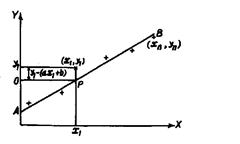
Let the observed values be given by (x^, y{), (X2, y2)……(*n. y«)-
The equation of the straight line is given by X =
ax + b, where a is constant representing the slope of the
line and b is constant representing the intercept on the
y-axis. Referring to Fig. 1.18, let AB be any arbitrary
straight line placed in relation to the observed points
yd> (*2> yd, – (*n> yn)- Using this line to predict the
value of yi from x\, we get point P. Thus the difference
of predicted value and the actual value will, therefore,
be yi – (axi + b). What is required is to choose the
best-fitting line with respect to the observed values by
the method of least squares. This is done by choosing a
line for which the sum of the squares of the deviations
from it measured vertically is a minimum.

i Fig. 1.18. Deviation of least-square line for two
dependent variables.
![]()
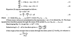
It is thus necessary to choose a and b to make E a minimum. This may be done by
differentiating expression partially with respect to a and b and then equating each derivative to
zero. Thus

![]()
3. Series of Observed Values of Three Dependent Variables. Such a problem arises in the
measurement of a surface table when the variations (z) from a truly flat plane are determined at a
number of positions (x, y) on the surface plane.
Let the observed values be given by (x-y yx, z{), (x^ y& z2), —. ten, zn)-
The equation of the flat plane is given by :
Z = ax + by + c.
Let any arbitrary plane be placed in relation to be observed points (xi, yi, zj), (x2, y2, z2)……,
ten, yn> zn). Using this plane to predict the value of zi from (xy, y{), we get a point N. Thus the
predicted value of Z\ =Z\= axi + by\ + c. The difference between the predicted value and the actual
value will therefore be :
zi – (axi + by i + c).
What is required is to choose the best-fitting plane with respect to the observed values by
the method of least squares. This is done by choosing a plane for which the sum of the squares of
the deviations from it measured vertically is a minimum.
![]()
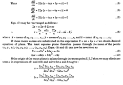
It is thus necessary to choose a, b and c to make E a minimum. This may be done by
differentiating the expression for E, partially with respect to a, b and c and then equating each
derivative to zero.

![]()
