Point Processing (Introduction to Video and Image Processing) Part 4

Automatic Thresholding: Global Method

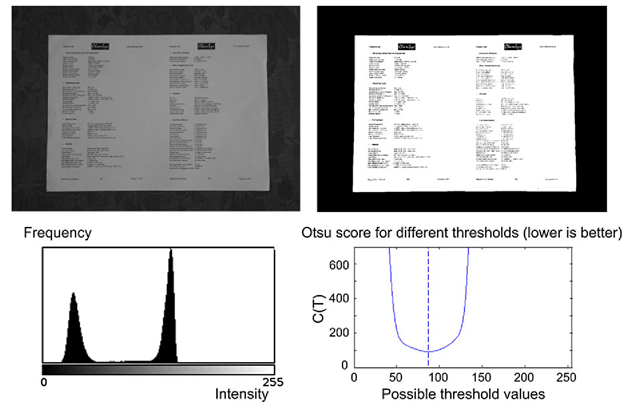
As mentioned above, thresholding is based on the notion that an image consists of two groups of pixels; those from the object of interest (foreground) and those from the background. In the histogram these two groups of pixels result in two “mountains” denoted modes. We want to select a threshold value somewhere between these two modes. Automatic methods for doing so exist and they are based on analyzing the histogram, i.e. all pixels are involved, and hence denoted a global method. The idea is to try all possible threshold values and for each, evaluate if we have two good modes. The threshold value producing the best modes is selected. Different definitions of “good modes” exits and here we describe the one suggested by Otsu [14].

The method evaluates Eq. 4.15 for each possible threshold value T and select the T where C(T) is minimum. The reasoning behind the equation is that the correct threshold value will produce two narrow modes, whereas an incorrect threshold value will produce (at least one) wide mode. So the smaller the variances the better. To balance the measure, each variance is weighted by the number of pixels used to calculate it.

Fig. 4.21 Global automatic thresholding. Top left: Input image. Top right: Input image thresh-olded by the value found by Otsu’s method. Bottom left: Histogram of input image. Bottom right: C(T) as a function of T. See text. The vertical dashed line illustrates the minimum value, i.e., the selected threshold value

A very efficient implementation is described in [14]. The method works very well in situations where two distinct modes are present in the histogram, see Fig. 4.21, but it can also produce good results when the two modes are not so obvious.

where M1(T) is the number of pixels to the left of T and M2(T) is the rest of the pixels in the image. σ2(T) and σ2(T) are the variances of the pixels to the left and right of T, respectively.

Automatic Thresholding: Local Method

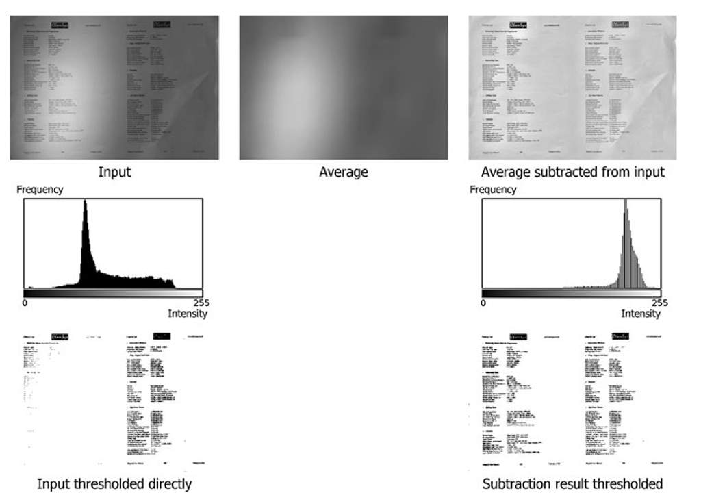
In Fig. 4.23 an image with non-even illuminating is shown. The consequence of this type of illumination is that an object pixel in one part of the image is identical to a background pixel in another part of the image. The image can therefore not be thresholded using a single (global) threshold value, see Fig. 4.23. But if we crop out a small area of the image and look at the histogram, we can see that two modes are present and that this image can easily be thresholded, see Fig. 4.22. From this follows that thresholding is possible locally, but not globally.

We can view thresholding as a matter of finding object pixels and these are per definition different from background pixels. So if we had an image of the background, we could then subtract it from the input image and the object pix- els would stand out.

Fig. 4.22 Left: Cropped image. Center: Histogram of input. Right: Thresholded image

Fig. 4.23 Local automatic thresholding. Top row: Left: Input image. Center: Mean version of input image. Right: Mean image subtracted from input. Center row: Histograms of input and mean image subtracted from input. Bottom row: Thresholded images

We can estimate a background pixel by calculating the average of the neighboring pixels.3 Doing this for all pixels will result in an estimate of the background image, see Fig. 4.23. We now subtract the input and the background image and the result is an image with a more even illumination where a global threshold value can be applied, see Fig. 4.23.4 Depending on the situation this could either be a fixed threshold value or an automatic value as describe above.

The number of neighborhood pixels to include in the calculation of the average image depends on the nature of the uneven illumination, but in general it should be a very high number. The method assumes the foreground objects of interest are small compared to the background. The more this assumption is violated, the worse the method performs.

Logic Operations on Binary Images

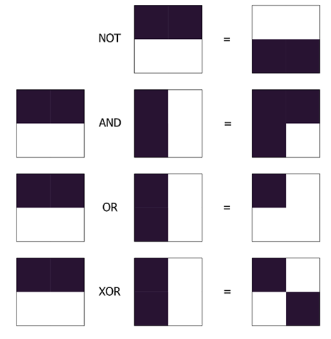
After thresholding we have a binary image consisting of only white pixels (255) and black pixels (0). We can combine two binary images using logic operations. The basic logic operations are NOT, AND, OR, and XOR (exclusive OR). The NOT operation do not combine two images but only works on one at a time. NOT simply means to invert the binary image. That is, if a pixel has the value 0 in the input it will have the value 255 in the output, and if the input is 255 the output will be 0. The three other basic logic operations combine two images into one output. Their operations are described using a so-called truth table. Below the three truth tables are listed.

A truth table is interpreted in the following way. The left-most column contains the possible values a pixel in image 1 can have. The topmost row contains the possible values a pixel in image 2 can have. The four remaining values are the output values. From the truth tables we can for example see that 255 AND 0 = 0, and 0 OR 255 = 255. In Fig. 4.24 a few other examples are shown. Note that from a programming point of view white can be represented by 1 and only one byte is then required to represent each pixel. This can save memory and speed up the implementation.

Image Arithmetic

Instead of combining an image with a scalar as in Eq. 4.1, an image can also be combined with another image. Say we have two images of equal size, f1(x, y) and f2(x, y). These are combined pixel-wise in the following way:

 

Fig. 4.24 Different logic operations

Other arithmetic operations can also be used to combine two images, but most often addition or subtraction are the ones applied. No matter the operation image arithmetic works equally well for gray-scale and color images.

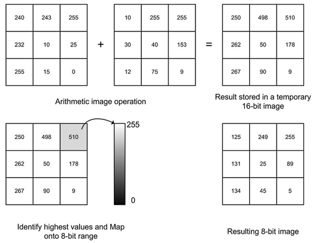
When adding two images some of the pixel values in the output image might have values above 255. For example if /1(10, 10) = 150 and /2(10, 10) = 200, then g(10, 10) = 350. In principle this does not matter, but if an 8-bit image is used for the output image, then we have the problem known as overflow. That is, the value cannot be represented. A similar situation can occur for image subtraction where a negative number can appear in the output image. This is known as underflow.

One might argue that we could simply use a 16 or 32-bit image to avoid these problems. However, using more bit per pixel will take up more space in the computer memory and require more processing power from the CPU. When dealing with many images, e.g., video data, this can be a problem.

The solution is therefore to use a temporary image (16-bit or 32-bit) to store the result and then map the temporary image to a standard 8-bit image for further processing. This principle is illustrated in Fig. 4.25.

This algorithm is the same as used for histogram stretching except that the minimum value can be negative:

1.    Find the minimum number in the temporary image, /1

2.    Find the maximum number in the temporary image, /2

3.    Shift all pixels so that the minimum value is 0: gi (x, y) = gi (x, y) – /

4.    Scale all pixels so that the maximum value is where gi (x, y) is the temporary image.

Fig. 4.25 An example of overflow and how to handle it. The addition of the images produces values above the range of the 8-bit image, which is handled by storing the result in a temporary image. In this temporary image the highest value is identified, and used to scale the intensity values down into the 8-bit range. The same approach is used for underflow. This approach also works for images with both over- and underflow

Image arithmetic has a number of interesting usages and here two are presented. In Chap. 8 we present another one, which is related to video processing.

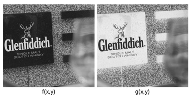
The first one is simply to invert an image. That is, a black pixel in the input becomes a white pixel in the output etc. The equation for image inversion is defined in Eq. 4.17 and an example is illustrated in Fig. 4.26.

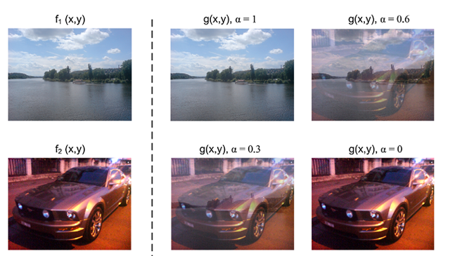
Another use of image arithmetic is alpha blending. Alpha blending is used when mixing two images, for example gradually changing from one image to another image. The idea is to extend Eq. 4.16 so that the two images have different importance. For example 20% of f1(x, y) and 80% of f2(x, y). Note that the sum of the two percentages should be 100%. Concretely, the equation is rewritten as

where α e [0, 1] and α is the Greek letter “alpha”, hence the name alpha blending. If α = 0.5 then the two images are mixed equally and Eq. 4.18 has the same effect as Eq. 4.16. In Fig. 4.27, a mixing of two images is shown for different values of α.

Fig. 4.26 Input image and inverted image

Fig. 4.27 Examples of alpha blending, with different alpha values

In Eq. 4.18, α is the same for every pixel, but it can actually be different from pixel to pixel. This means that we have an entire image (with the same size as f1(x, y), f2(x, y) and g(x, y)) where we have α-values instead of pixels: α(x, y). Such an “α-image” is often referred to as an alpha-channel. This can for example be used to define the transparency of an object.