Neighborhood Processing (Introduction to Video and Image Processing) Part 2

Correlation

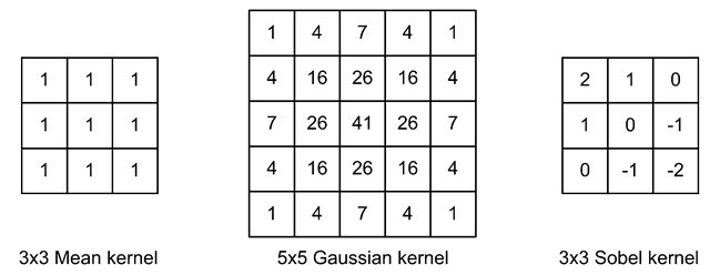
Correlation is an operation which also works by scanning through the image and applying a filter to each pixel. In correlation, however, the filter is denoted a kernel and plays a more active role. First of all the kernel is filled by numbers—denoted kernel coefficients. These coefficients weight the pixel value they are covering and the output of the correlation is a sum of weighted pixel values. In Fig. 5.6 some different kernels are shown.

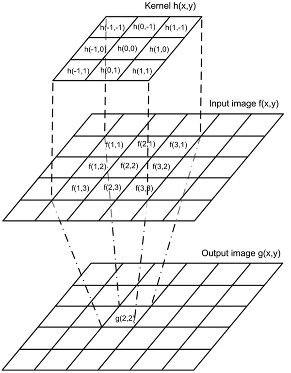
Similar to the median filter the kernel is centered above the pixel position whose value we are calculating. We denote this center (0, 0) in the kernel coordinate system and the kernel as h(x, y), see Fig. 5.7. To calculate the output value we take the value of h(-1, -1) and multiply it by the pixel value beneath. Let us say that we are calculating the output value of the pixel at position (2, 2). Then h(-1, -1) will be above the pixel f(1,1) and the value of these two pixels are multiplied together. The result is added to the product of the next kernel element h(0, -1) and the pixel value beneath f (2,1), etc.

Fig. 5.6 Three different kernels

The final value which will be written into the output image as g(2, 2) is found as

The principle is illustrated in Fig. 5.7. We say that we correlate the input image f(x,y) with the kernel h(x,y) and the result is g(x,y). Mathematically this is expressed as g(x,y) = f(x,y) ◦ h(x,y) and written as

where R is the radius of the kernel.3 Below, a C-code example of how to implement correlation is shown:

 

 

 

 

Fig. 5.7 The principle of correlation, illustrated with a 3 x 3 kernel on a 6 x 6 image

When applying correlation, the values in the output can be above 255. If this is the case, then we normalize the kernel coefficients so that the maximum output of the correlation operation is 255. The normalization factor is found as the sum of the kernel coefficients. That isFor    the    left-most    kernel    in    Fig.    5.6 the normalization factor becomes 1 + 1 + 1 + 1 + 1 + 1 + 1 + 1 + 1 = 9, and the resulting kernel coefficients are 1 /9 as opposed to 1.

Fig. 5.8 An example of how a mean filter can be used to hide the identity of a person. The size of the mean kernel decides the strength of the filter. Actual image size: 512 x 384

Looking back on the previous section we can now see that the left-most kernel in Fig. 5.6 is exactly the mean filter. The mean filter smooths or blurs the image which has different applications. In Fig. 5.8 one application is shown where the mean filter is applied within the white box in order to hide the identity of a person. The bigger the kernel, the more the smoothing. Another type of mean filter is when a kernel like the middle one in Fig. 5.6 is applied. This provides higher weights to pixels close to the center of the kernel. This mean filter is known as a Gaussian filter, since the kernel coefficients are calculated from the Gaussian distribution (a bell-shaped curve).

Template Matching

An important application of correlation is template matching. Template matching is used to locate an object in an image. When applying template matching the kernel is denoted a template. It operates by defining an image of the object we are looking for. This object is now the template (kernel) and by correlating an image with this template, the output image indicates where the object is. Each pixel in the output image now holds a value, which states the similarity between the template and an image patch (with the same size as the template) centered at this particular pixel position. The brighter a value, the higher the similarity.

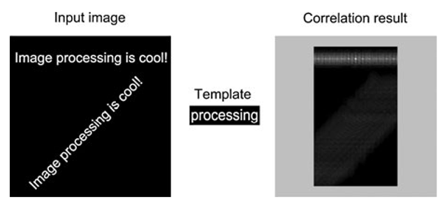
In Fig. 5.9 the correlation-based template matching is illustrated.4 We can see a bright spot in the center of the upper part of the output corresponding to where the template matches best. Note also that as the template is shifted left and right with respect to this position, a number of bright spots appear. The distances between these spots correspond to the distance between the letters in the text.

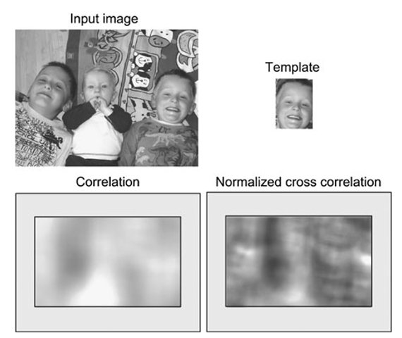
Since correlation is based on multiplying the template and the input image, bright areas in the input image tend to produce high values in the output. This is illustrated in Fig. 5.10 where the large white section in the clothing of the child in the middle produces the highest values in the output. This problem in general makes it difficult,and in this particular case impossible, to actually find the position of the object by looking at the values in the output image.

Fig. 5.9 Template matching performed by correlating the input image with a template. The result of template matching is seen to the right. The gray outer region illustrates the pixels that cannot be processed due to the border problem

Fig. 5.10 Template matching using correlation and normalized cross-correlation. The gray regions illustrate the pixels that cannot be processed due to the border problem

To avoid this problem we need to normalize the values in the output so they are independent of the overall level of light in the image. To assist us in doing so we use a small trick. Let us denote the template H and the image patch F. These are both matrices, but by rearranging we can easily convert each matrix into a vector by concatenating each row (or column) in the matrix, i.e., ~H and ~F.

If we now look at correlation in terms of this vector representation, we can see that Eq. 5.4 is actually the dot product between the two vectors.From geometry we know that the dot product between two vectors can be normalized to the interval [-1, 1] using the following equation:

where θ is the angle between the two vectors, and \Ή| and |"^| are the lengths of the two vectors. The normalization of the dot product between the vectors is a fact because cos θ e [-1,1]. The length of |Ή\, which is also the “length” of the template, is calculated as

where R is the radius of the template and h(i, j) is the coefficient in the template at position (i, j). The length of the image patch is calculated in the same manner.

When using this normalization the bright spots in the output no longer depend on whether the image is bright or not but only on how similar the template and the underlying image patch are. This version of template matching is denoted normalized cross-correlation (NCC) and calculated for each pixel (x, y) using the following equation:

where R is the radius of the template, H = h(i, j) is the template and F = f(x + i,y + j) is the image patch. cos θ e [-1,1] but since the image patch and the template always contain positive numbers, cos θ e [0,1], i.e., the output of normalized cross-correlation is normalized to the interval [0, 1], where 0 means no similarity and 1 means a complete similarity. In Fig. 5.10 the benefit of applying normalized cross-correlation can be seen.

An even more advanced version of template matching exist. Here the mean values of the template and image patch are subtracted from H and F, respectively. This is known as the zero-mean normalized cross-correlation or the correlation coefficient. The output is in the interval [-1,1] where 1 indicates a maximum similarity (as for NCC) and -1 indicates a maximum negative similarity, meaning the same pattern but opposite gray-scale values: 255 instead of 0, 254 instead of 1, etc.

Independent of the type of template matching, the kernel (template) is usually much bigger than the kernels/filters used in other neighborhood operations. Template matching is therefore a time consuming method and can benefit from introducing a region-of-interest, see Sect. 2.4.1.

A general assumption in template matching is that the object we are looking for has roughly the same size and rotation in both the template and the image. If this cannot be ensured, then we need to have multiple scaled and rotated versions of the template and perform template matching using each of these templates. This requires significant resources and the speed of the system is likely to drop.

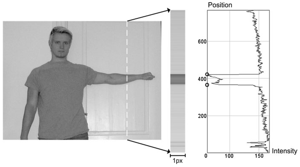
Fig. 5.11 A single column of the image is enlarged and presented in a graph. This graph contains two very significant changes in height, the position of which is marked with circles on the graph. This is how edges are defined in an image

Edge Detection

Another important application of correlation is edge detection. An edge in an image is defined as a position where a significant change in gray-level values occur. In Fig. 5.11 an image is shown to the left. We now take an image slice defined by the vertical line between the two arrows. This new image will have the same height as the input image, but only be one pixel wide. In the figure this is illustrated. Note that we have made it wider in order to be able to actually see it. Imagine now that we interpret the intensity values as height values. This gives us a different representation of the image, which is shown in the graph to the right.

What can be seen in the graph is that locations in the original image where we have a significant change in gray-scale value appear as significant changes in height. Such positions are illustrated by circles in the figure. It is these positions where we say we have an edge in an image.

Edges are useful in many applications since they define the contour of an object and are less sensitive to changes in the illumination compared to for example thresholding. Moreover, in many industrial applications image processing (or rather machine vision) is used to measure some dimensions of objects. It is therefore of great importance to have a clear definition of where an object starts and ends. Edges are often used for this purpose.