Modelling Three-Dimensional Objects (Introduction to Computer Graphics Using Java 2D and 3D) Part 3

Representation of Functions in Java 3D

The representation of landscapes and functions of two variables in Java 3D can be implemented directly based on the class GeometryArray which has been introduced in Sect. 6.4. In the simplest case of a rectangular grid, one only needs to combine the coordinates of the grid points with the corresponding altitude information of the landscape or with the value of the function at the corresponding point to define the points for the GeometryArray. Each rectangle of the grid is then split into two triangles and the corresponding triangles in 3D are obtained when the altitude information is taken into account.

The representation of the function z = x sin(7x) cos(4y) in Fig. 6.13 on page 142 was generated using the class SurfaceExample.java. The method createSurface is implemented in this class. This method computes a corresponding GeometryArray for a given function of two variables. With this GeometryArray a Shape can be created that can be included in a scenegraph. The method createSurface requires a number of parameters.

•    The function to be displayed must be an implementation of the Interface1 IFunctionInTwoVariables. The interface must be implemented in a concrete class. The class FunctionInTwoVariablesExample that realises the function z = x sin(7x) cos(4y) is an example for the implementation of this Interface.

•    The following four values define the range [IffiiillImax] x [ymm,ymax] over which the function should be plotted. The two values after these four values can be used to limit the range of the function values, i.e. the z-values. In order to apply this limited range cutting of smaller and larger values, the Boolean value after these two values must be set to true. Otherwise the function will be drawn over the whole rectangle, no matter how small or large the z-values are.

•    The next six parameters define a box within which the function should be drawn in the virtual 3D-world or within the transformation group. This box should normally be centred around the origin, even if the function is defined over a range like [1000, 2000] x [1000, 2000].

•    The last two parameters specify how many grid points should be used in x- and y-direction for the approximation of the surface by triangles.

Text in 3D

Text in a virtual 3D-world can be two-dimensional, i.e. flat, or three-dimensional. Two-dimensional letters are usually mapped onto surfaces as textures which will be discussed in Sect. 8.8. Such text or letters can, for instance, occur on posters or road signs in a scene. 3D-letters are modelled as geometric objects. A possible application of 3D-letters could be illuminated advertising.

Three-dimensional text can also be used for the labelling and legends in graphics. Displaying a function of two variables requires three dimensions—two for the input variables and one for the output variable—and the axes need to be labelled. Two problems can occur when the user is allowed to navigate in such a scene in order to view the function of two variables from different angles. The first one is that the labelling or the legends can become too small and unreadable when zooming out of the scene to a very far distance. The second problem caused by the navigation is that the 3D-letters are difficult to read or cannot be read anymore when they are seen from the side or from the back.

In order to avoid these problems, suitable transformations can be applied to the letters so that they always occur in the same size independent of the distance to the viewer and that they are always oriented to the viewer. The latter technique is called billboard behaviour.

Text in Java 3D

Java 3D offers the classes Text2D and Text3D for the representation of two- and three-dimensional text in a scene. Text2D maps the text as texture onto a virtual transparent rectangle. The text can only be seen from the front. Three-dimensional text can be generated by Text3D yielding letters that are visible from all angles, but they might not be readable under an unfavourable angle. As an example for text in a 3D scene, we consider the class Text3D. Text2D is used in a similar way.

In order to include a three-dimensional text in a scene, a suitable font f as instance of the class Font must be defined as it is already described in Sect. 4.4. The following program code generates a text consisting of three-dimensional symbols:

The first line turns the ordinary Font f— f must be defined before—into a threedimensional Font3D f3d. The object FontExtrusion determines how the three-dimensional font is derived from the two-dimensional one. Then an object Text3D t3d is generated, containing the text in the form of a String s and the specification of a Point3f p is required in order to position the text. This Text3D-object can then be used together with an Appearance app to generate a Shape3D-object which can be included in the scenegraph or a transformation group.

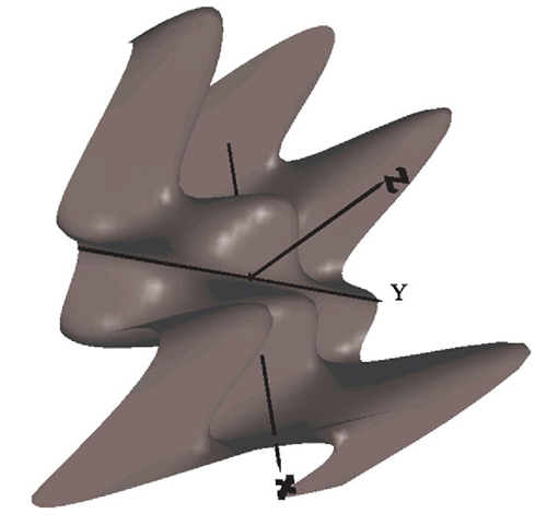
Fig. 6.16 Labels for the axes: A Billboard behaviour is used only for the letter Y

If a text or—more generally—any object or transformation group should always be oriented to the viewer, no matter from which angle the scene is viewed, this can be achieved by using a Billboard behaviour. An instance of the class Billboard must be created. The transformation group tgBBGroup which should always be oriented to the viewer must be one of the arguments in the constructor of the Billboard object. As a second argument, a constant is needed to specify which transformation should be applied to orient the transformation group to the user. In the following example, the constant is chosen as Billboard.ROTATE_ABOUT_POINT, meaning that the orientation of the transformation group is based on a rotation around a point. Finally, the point around which the rotation should take place must be specified in the form of an object

A bounding region must be assigned to the Billboard behaviour, for instance in the form of a BoundingSphere bounds. Furthermore, the Billboard behaviour must be assigned to the corresponding transformation group tgBBGroup. It is necessary to allow changing of the transformation of the corresponding transformation group, so that the Billboard behaviour can orient the transformation group to the viewer.

The program Text3DExample.java extends the visualisation of the function in the program SurfaceExample.java by a coordinate system with labels for the axes. A Billboard behaviour is only used for the label of the y-axis. Figure 6.16 shows the result after rotating the view. The labels for the x- and the z-axis are not oriented to the viewer, whereas the letter Y is oriented to the viewer by the use of the Billboard behaviour.

Parametric Curves and Freeform Surfaces

For the representation of a scene as an image, the surfaces of geometric objects are approximated by triangles. But an explicit description of surfaces with triangles is not suitable for modelling. Freeform surfaces are much better suited for this purpose. They are the three-dimensional counterpart of curves in the plane as described in Sect. 2.3. Like these curves, a freeform surface is defined by a finite set of points which it approximates. Saving geometric objects based on freeform surfaces does not cause any problems when the object is scaled. Tesselations are not well suited for scaling an objects. They will lead to similar problems as scalings of raster graphics. For a given freeform surface, the number of triangles for the tesselation can be chosen depending on the desired precision and resolution. The freeform surfaces provide also exact information about the normal vectors to the surface which are very important for illumination and shading.

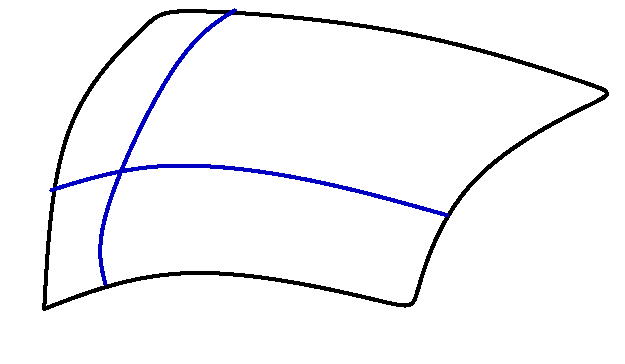
Modelling curved surfaces is based on parametric curves. When a surface is scanned parallel to one of the coordinate axes, one obtains a curve in the threedimensional space. Figure 6.17 shows two curves that are obtained from scanning a surface. Understanding parametric curves in the three-dimensional space is essential for the understanding of curved surfaces. Therefore, a brief introduction to parametric curves is given, before freeform surfaces are discussed.

Parametric Curves

When a curve in the three-dimensional space or in the plane should be defined by a finite set of points—the so-called control points—the following properties will make modelling and adjusting such curves easier.

Controllability: The influence of the parameters on the shape of the curve can be understood in an intuitive way. When the shape of a curve has to be changed, it should be clear for the user which parameters he should modify in which way in order to achieve the desired change.

Locality principle: It must be possible to carry out local changes on the curve. Modifying one control point should only change the curve in the neighbourhood of this control point and not alter the curve completely.

Smoothness: The curve should satisfy certain smoothness properties. It should not only be continuous without jumps, it should have no sharp bends. The latter property requires the curve to be differentiable. In some cases it is even necessary that higher derivatives exist. It also desirable that the curve is of bounded variation. This means it should stay somehow close to its control points.

Fig. 6.17 Two curves obtained from a surface that is scanned along the coordinate axes

Interpolation refers to curves that pass through all control points whereas approximation only requires that the curve gets close to the control points, but it does not have to pass through them. Given (n + 1) control points, there is always an interpolation polynomial of degree n or less that passes exactly through the control points. Nevertheless, interpolation with polynomials is not suited for the modelling purposes of computer graphics. Apart from the problem that the evaluation of polynomials of higher degree leads to high computational costs, interpolation polynomials do not satisfy the locality principle. The modification of a single control point usually affects all coefficients of the polynomial and changes the whole curve. Clipping for such polynomials is also not easy, since a polynomial interpolating a given set of control points can deviate arbitrarily from the region around the control points. Therefore, it is not sufficient to consider only the control points for clipping of such interpolation polynomials. The curve must be computed directly to check whether it passes through the clipping area. Another problem of polynomials of higher degree is that they tend to oscillate between the control points.

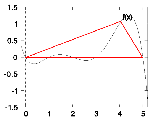
Figure 6.18 shows an interpolation polynomial of degree 5, defined by six control points through which it passes. With the exception of one control point, all others are located on the x-axis. The polynomial oscillates around the control points and has a clear overshoot above the highest control point. It does not stay within the convex hull of the control points.

The undesired properties of interpolation polynomials can be amended by dropping the strict requirement that the polynomial must pass through all control points. Instead, it is sufficient to approximate some of the control points only. Bernstein polynomials of degree n are a class of polynomials with better properties than interpolation polynomials. The ith Bernstein polynomial of degree n (i e(0,…,n|) is given by the equation

Bernstein polynomials satisfy two important properties.

Fig. 6.18 An interpolation polynomial of degree 5 defined by the control points (0, 0), (1,0), (2, 0), (3, 0), (4, 1), (5,0)

This means that the evaluation of a Bernstein polynomial within the unit interval will only yield values between zero and one. This property and the following one will be needed later on for constructing curves that stay within the convex hull of their control points:

In every position of the unit interval the Bernstein polynomials add up to one.

Bézier curves use Bernstein polynomials of degree n to approximate (n + 1) control points b0,…, bn e . For the purposes of computer graphics only the cases of the plane with p = 2 and the three-dimensional space with p = 3 are of interest. The control points are also called Bézier points. The curve

defined by these points is called a Bézier curve of degree n.

The Bézier curve interpolates the first and the last point, this means x(0) = b0 and x(1) = bn hold. In general, the curve does not pass through the other control points. The tangent vector to the Bézier curve in the first and the last point can be calculated in the following way:

This means that the tangent vector in the first point b0 points in the direction of the point b1 and the tangent vector in the last point bn points in the direction of the point bn-i. This principle is already known from the definition of cubic curves in Fig. 2.7 on page 14.

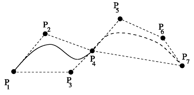
Fig. 6.19 B-spline with knots P1, P4, P7 and inner Bézier points P2, P3, P5, P6

Fixing the value t in (6.3), one obtains a convex combination of the control points b0,…, bn, since the values x(t) of the Bernstein polynomials add up to one in every point t. Therefore, the Bézier curve stays within the convex hull of the control points.

When an affine transformation is applied to the control points, the resulting Bézier curve with respect to the new control points coincides with the transformed Bézier curve. Therefore, Bézier curves are invariant under affine transformations like rotation, translation or scaling. Bézier curves are also symmetric with respect to their control points. The control points b0,…, bn and bn,…, b0 lead to the same curve. The curve is only passed through in the reverse direction.

When a convex combination of two sets of control points is used to define a new set of control points, then the resulting Bézier curve is the convex combination of the corresponding Bézier curves.

•    If the control points Ib0,…, Ibn define the Bézier curve X(t) and

•    the control points Ib0,…, Ibn define the Bézier curve X(t),

•    then the control points ab0 + βlb0,…,albn + βIbn define the Bézier curve x(t) = aX(t) + βX(t) if α + β = 1, α,β > 0 holds.

When all control points lie on a line or a parabola, then the resulting Bézier curve will be the corresponding line or parabola. Bézier curves also preserve certain geometrical shape properties like monotonicity or convexity of the control points.

Despite the nice properties of Bézier curves, they are not suited for larger sets of control points since this would lead to polynomials of high degree. (n + 1) control points usually define a Bézier curve which is a polynomial of degree n. Therefore, instead of Bézier curves, B-splines are preferred to define approximating curves for a given set of control points. B-splines are composed of a number of Bézier curves of lower polynomial degree—usually degree three or four. For this purpose, for a sequence of n control points (for instance n = 4) a Bézier curve is computed and the last control point of the sequence is used as the starting point of the next sequence for the next Bézier curve. In this way, B-splines interpolate those control points where the single Bézier curves are glued together. These junctions are also called knots. The other control points are called inner Bézier points. Figure 6.19 shows a B-spline which is composed of two Bézier curves of degree 3.

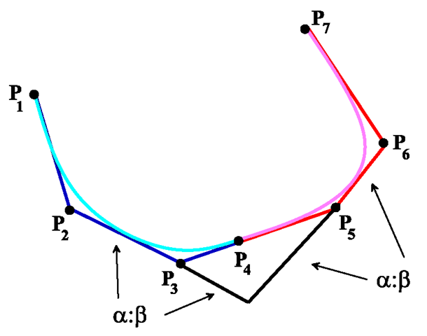
Fig. 6.20 Condition for the inner Bézier points for a twice differentiable, cubic B-spline

In order to avoid sharp bends at junctions between the Bézier curves, each knot and its two neighbouring inner Bézier points should be collinear. In this way, the B-spline will be differentiable also in the knots. This method for avoiding sharp bends was illustrated in Fig. 2.8 on page 14. By choosing the inner Bézier points properly, a B-spline of degree n can be differentiated (n – 1) times. Cubic B-splines are based on polynomials of degree three and can therefore be twice differential when the inner Bézier points are chosen correctly. In addition to the collinearity condition, another restriction must be imposed on the neighbouring inner Bézier points. The B-spline in Fig. 6.20 is composed of two Bézier curves of degree 3. It is defined by the knots P1, P4, P7 and the inner Bézier points P2, P3, P5, P6. In order to guarantee that the B-spline is twice differentiable, the segments of the tangents must have the same proportions as indicated in Fig. 6.20.

B-splines preserve the nice properties of Bézier curves. They stay within the convex hull of the control points, they are invariant under affine transformations, symmetric in the control points, they interpolate the first and the last control point and they satisfy the locality principle.

A B-spline is piecewise composed of Bézier curves. They can be described in homogeneous coordinates in the form

Px(t), Py(t), Pz(t) are polynomials in t. When a perspective projection in the form of a matrix as in (5.6) is applied to this representation of a Bézier curve, one obtains

Therefore, the projection of a Bézier curve as a parametric curve is no longer a polynomial in Cartesian coordinates, but a rational function.

Since a perspective projection of a B-spline or a Bézier curve will lead to a rational function anyway, one can already use rational functions for modelling curves in the three-dimensional space. The perspective projection of a rational function is again a rational function. Therefore, it is very common to use NURBS (nonuniform rational B-splines) instead of B-spline. NURBS are generalisations of B-splines based on extensions of Bézier curves to rational functions in the following form:

The adjustable weights wi are called form parameters. A larger weight wi increases the influence of the control point bi on the curve. For support of this interpretation and to avoid singularities, it is usually required that all weights Wi are positive.