Drawing Lines and Curves (Introduction to Computer Graphics Using Java 2D and 3D) Part 3

The Midpoint Algorithm for Circles

In Sect. 3.2 an efficient line drawing algorithm based solely on integer arithmetic was introduced. This midpoint algorithm can be generalised to drawing circles and also various other curves under certain restrictions. The main constraint for circles is that the centre or midpoint (xm,ym) of the circle must be located on a pixel, i.e., xm and ym must be integer values. In this case, it is sufficient to develop an algorithm for drawing circles centred around the origin of the coordinate system. For circles with midpoint (xm,ym) the same algorithm can be applied as for circles with midpoint (0, 0), but all points are drawn with an offset of (xm,ym).

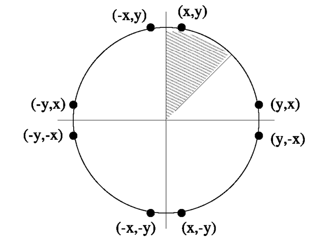
Fig. 3.17 Exploiting symmetry for drawing circles

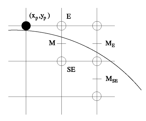
Fig. 3.18 Midpoint algorithm for circles

In order to determine the pixels to be drawn for a circle centred around the origin of the coordinate system, the calculations are only carried out for an eighth part of the circle. The other pixels can be derived directly by symmetry arguments as Fig. 3.17 shows. If the pixel (x, y) has to be drawn within the considered hatched eighth part of the circle, then the pixels (±x, ±y) and (±y, ±x) have to be drawn in the other parts of the circle.

For the generalisation of the midpoint or Bresenham algorithm to circles [2], another constraint is introduced. It is assumed that the radius R is integer-valued. In the considered eighth part of the circle, the slope of the circle line decreases from 0 to —1. Analogously to the case of drawing lines with a slope between zero and one, the number of candidates for the next pixel to be drawn can be reduced to two. If the pixel (xp,yp) has been drawn in one step, the next pixel can only be the pixel E with coordinates (xp + 1,yp) or SE with coordinates (xp + 1,yp — 1) as is illustrated in Fig. 3.18.

In the same way as in the case of the midpoint algorithm for lines, the decision which pixel is the correct one to be drawn in the next step is based on a decision variable involving the midpoint between the two pixel candidates. For this purpose, the equation for the circle x2 + y2 = R2 is rewritten in the form

For this implicit equation and a point (x, y) the following statements are obvious:

In order to decide whether pixel E or SE is the next pixel to be drawn, the midpoint M is inserted into (3.13) leading to the following decisions:

•    If d > 0 holds, then SE must be drawn.

•    If d < 0 holds, then E must be drawn.

As in the case of the midpoint algorithm, the value of the decision variable d is not computed in each step by inserting the midpoint M directly. Instead, only the change of d is calculated in each step. Starting with pixel (xp,yp) which is assumed to be drawn correctly, the change of d is calculated for the transition from pixel (xp+1,yp+1 ) to (xp+2,yp+2). Two cases must be distinguished here.

Case 1: E, i.e., (xp+1,yp+1) = (xp + 1,yp) was the pixel drawn after (xp,yp). This corresponds to the case shown in Fig. 3.18. The midpoint ME to be considered for drawing the pixel (xp+2,yp+2) has the coordinates (xp + 2,yp — 1 ). Inserting this midpoint into (3.13) yields the following value for the decision variable d:

In the previous step for determining the pixel (xp+1,yp+1), the midpoint (xp + 1,yp + 1 ) was considered. Inserting this midpoint into (3.13) gives

as the previous value for the decision variable d. The change of the decision variable is in this case

Case 2: SE, i.e.,was the pixel drawn after (xp,yp).

In this case, the next midpoint to be considered is.(see Fig. 3.18). Then the value for the decision variable is

The previous value of d is the same as in the case of the pixel E, so that the change of the decision variable is given by

Taking these two cases together, the change of the decision variable is

This means

so that the change Δ of the decision variable d is always an integer value.

In order to compute the decision variable d in each step, in addition to its change the initial value is also needed. The first pixel to be drawn has the coordinates (0,R), so that (1,R — 1 ) is the first midpoint to be considered. The initial value for d is therefore

As in the case of lines, the change of the decision variable is always integer-valued, but the initial value is not. The same principle as for lines could be applied to circles. Using the modified decision variable D = 4 · d would resolve the problem of the initial floating point value. A simpler solution is, however, to simply ignore the resulting digits after the decimal dot in (3.14) for the initialisation of d. The reason why this does not lead to any mistakes for the drawing of the circle is very simple. In each step, it is only of interest whether d has a positive or a negative value. Since d will always be changed by an integer value, the sign of d is the same with or without the digits after the decimal dot.

For the derivation of the midpoint algorithms for drawing circles it was assumed that the centre of the circle is in the origin of the coordinate system or at least a point on the pixel raster. In addition, the constraint that the radius must have an integer value was introduced. The midpoint algorithm can be extended easily to circles with an arbitrary, not necessarily integer-valued radius. Since the radius does not occur in the update equations for the decision variable d, the radius must only be considered for the initialisation of d. For a floating point radius R the first pixel to be drawn is (0, round(R)), leading to (1, round(R) — 2) as the first midpoint that must be considered. Therefore, d must be initialised with the value

For the same reasons as for circles with an integer-valued radius, the digits after the decimal dots can be ignored. This makes the initialisation of d integer-valued and the change of d remains integer-valued independent of the radius.

Drawing Arbitrary Curves

The midpoint algorithm can be generalised not only to circles, but also to other curves, for instance ellipses [10, 11, 13]. A very restrictive requirement of the midpoint algorithm is that the slope of the curve to be drawn must lie between 0 and 1 or between 0 and —1. For drawing arbitrary curves, or at least continuous curves, the plot of the graph is based on piecewise approximations of the curve by short lines. For drawing the continuous function y = f(x) it is not sufficient to iterate stepwise through the x -values and draw the corresponding pixel with the rounded y-coordinate. Whenever the function has an absolute slope larger than one, the same problem of pixel gaps occurs as already happened with the naïve line drawing algorithm in Fig. 3.2 on page 44. Lines have a constant slope that can be determined easily. Therefore, the problem of pixel gaps can be avoided for lines by simply exchanging the roles of the coordinate axes for drawing a line with an absolute slope greater than one. This means that in this case the inverse function of the line is drawn along the y-axis. Arbitrary functions have neither a constant slope, nor can the slope or the inverse function be calculated easily for arbitrary functions. For this reason, drawing arbitrary curves is carried out by stepwise iterating through the desired range on the x-axis and computing the corresponding rounded y -values. However, not only these pixels are drawn, but also the connecting line between pixels with neighbouring x-values is drawn based on the midpoint algorithm for lines.

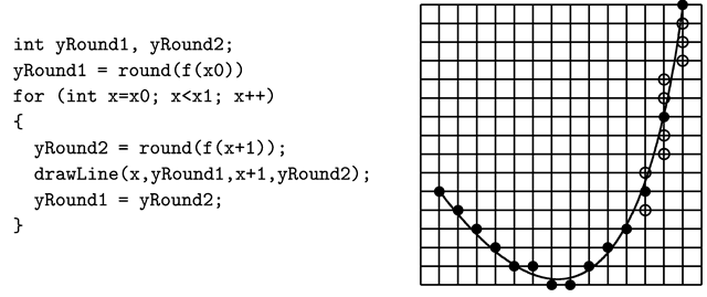
Figure 3.19 illustrates the principle for drawing a continuous function y = f(x) in the interval [x0 ,x1 ] with x0 ,x1 G N. The filled circles are the pixels of the form (x, round(f (x))) for integer-valued x-coordinates. The empty circles correspond to the pixels that are drawn when two of the computed pixels with neighbouring x -coordinates shown as full circles are connected by a line. Drawing a curve in this way might not lead to exactly the same pixels that would result if always the closest pixel to the curve was chosen. However, the deviation is at most one pixel.

Fig. 3.19 Drawing arbitrary curves

Antialiasing

The term aliasing effect originates from the field of signal processing and refers to phenomena that occur when a continuous signal is sampled in a discrete manner with a constant rate. Drawing a line or curve is a similar procedure. The ideal line or curve as a continuous function is sampled by the pixel raster. The most common aliasing effects in computer graphics are the staircasing effects that occur when continuous curves or objects with smooth boundaries are mapped to a pixel raster. Assuming that lines must have a width of only one pixel and pixels can only be black or white, nothing can be done to avoid aliasing effects.

For grey-scale images or images that allow colour intensities, aliasing effects can be reduced. The basic idea of reducing staircasing effects for drawing lines and curves is to soften the boundaries of the line by decreasing the intensity. This technique is called antialiasing, for which various approaches are available. Some of these approaches are outlined in the following, explaining their principles for drawing lines.

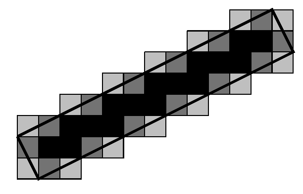
Unweighted area sampling interprets a line as a long, but very thin rectangle. A pixel is not understood as a point, but as a small square that can be filled with colour. The intensity of the pixel is chosen proportionally to the area of the pixel’s square that is covered by the rectangle that represents the line. Figure 3.20 illustrates this concept.

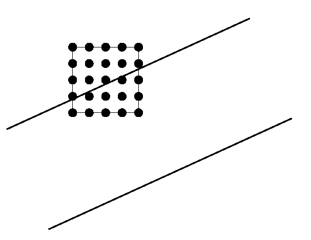
The main disadvantage of this method is that for each pixel’s square the intersection with a rectangle representing the line must be determined and the area of this intersection must be computed, requiring high computational costs. A simple heuristic approach to estimate the proportion of the pixel’s square that is covered by the line rectangle uses an imaginary refined pixel grid on each pixel’s square. The proportion of refined pixels in the square that also lie in the line rectangle gives a good estimation for the desired intensity of the pixel. In this way, the pixel whose refined 5 x 5 pixel grid is shown in Fig. 3.21 would obtain an intensity equal to 11/25.

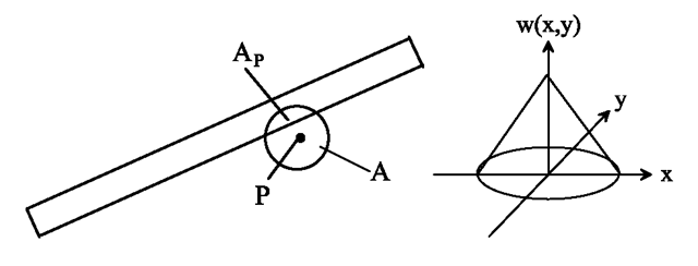
Weighted area sampling does not only consider the area of the pixel’s square that is covered by the line rectangle, but takes also a weighting function w(x, y) into account. w(x,y) has the highest value in the centre of the pixel and decreases with increasing distance. A typical weighting function is shown in Fig. 3.22. The weighting function is defined on a circle A around pixel P as can be seen in the left part of the figure. The intensity for the pixel is given by

where Ap is the intersection of the circle with the line rectangle. 

Fig. 3.20 Unweighted area sampling

Fig. 3.21 Estimation of the area by sampling with refined pixels

Although this formula might appear complicated and computationally inefficient, since integrals are involved, the intensity of the pixel depends only on its distance to the ideal line, at least when a weighting function is used as illustrated in the right part of Fig. 3.22. The intensity can be written as a function I(dP) where dP stands for the distance of pixel P to the line. The number of displayable intensity values is usually limited, for computer screens by 256. Instead of considering the real function I : [0, œ) — [0,1], it is sufficient to restrict to a discrete version I :[0, œ) —> |0,...,ïmax} of the function, when the available levels of intensities are 0,...,fmax. Scanning the pixel raster in the neighbourhood of the line in order to determine the intensity for each pixel, means that for each pixel a corresponding value of I must be computed. This task is related to the problem of drawing a line or curve y = f(x) on a pixel raster. For drawing a line, the procedure scans the pixel raster step by step—in this case only along one of the coordinate axes—and determines the corresponding rounded value of the function round(f (x)). The differences versus antialiasing are that the pixel raster is not only scanned along a coordinate axis, but in the neighbourhood of a line and that the discrete value I to be determined is not the y-value of the pixel to be drawn, but the corresponding discretised intensity value. Based on this analogy, the concept of the midpoint algorithm was also extended to antialiasing, requiring only integer arithmetic to determine the discrete intensity value. Examples for such antialiasing techniques are Gupta-Sproull antialiasing [8] and the algorithm of Pitteway and Watkinson [12]. For a detailed description of these algorithms the reader is referred to the original work [8, 12] or to [7, 9].

Fig. 3.22 Weighted area sampling

Antialiasing with Java 2D

In Java 2D the method

will make sure that all Shape and area objects, i.e., all objects that do not represent text, are drawn using antialiasing.

To apply antialiasing to drawing text, the method must be called with the following parameters:

Drawing Thick Lines

Today’s output devices have a high resolution, which leads to very thin lines, when lines are rendered with only one pixel as their width. Various techniques for drawing thick lines with a thickness of more than one pixel are available. The simplest approach is pixel replication. For drawing a curve with a slope between — 1 and 1, with each pixel the n pixels below and above are also drawn, so that the curve has a thickness of 2n + 1 pixels in the y-direction. The same effect that lines with larger slope look thinner as was demonstrated in Sect. 3.4 occurs here as well. It was mentioned in Sect. 3.1 that for drawing lines with an absolute slope larger than one the roles of the coordinate axes should be exchanged. Even for drawing arbitrary curves, this technique will be applied as was explained in Sect. 3.7. This is the reason why only lines with slope between — 1 and 1 are considered here. The principle of pixel replication is illustrated in the left-hand side of Fig. 3.23. The right part of the figure shows the moving pen technique. For drawing a pixel a thick pen with a tip of for instance 5 x 5 pixels is used, so that in addition to the pixel in the centre all other pixels belonging to the tip of the pen are also drawn.

Pixel replication can be viewed as a special case of the moving pen technique where the tip has a rectangular shape with a width of one pixel in one direction. As in the case of pixel replication, a line with higher slope up to an absolute slope of one will look thinner when a squared tip is used for the moving pen technique.

Fig. 3 .23 Pixel replication and the moving pen technique

Fig. 3.24 Different line endings and joins

In order to avoid drawing the same pixel multiple times in the case of the moving pen technique, the shape of the tip should be taken into account. For the tip in Fig. 3.23 consisting of 5 x 5 pixels and a line with a slope between zero and one, all 25 pixels have to be drawn in the first step. In the following steps, only the five pixels to the right, in case the right (eastern) pixel is the next pixel for the line, or nine pixels must be drawn, when the north-eastern pixel is the next pixel of the line.

Another strategy for drawing thick lines considers the lines as thin rectangles or, more generally, as polygons that have to be filled. Techniques for filling polygons will be the topic of the next topic.

When thick lines are drawn, line endings and joins in polylines can be modelled in different ways. Simple pixel replication results in lines whose endings are always parallel to one of the coordinate axes. This problem can be solved when the lines are considered as filled rectangles. But this leads to other problems at the joins for polylines. Figure 3.24 shows different ways line endings and joins between thick lines could be drawn. The thickness of the lines is exaggerated in the figure in order to display the effects clearly. In the leftmost part of the figure lines are considered as rectangles leading to an undesired effect where two lines meet. For the other three cases in the figure this bad effect is amended in three different ways. A prolongation of the outer lines of the rectangles until they meet as in the second case in Fig. 3.24 produces a sharp tip. For the next image, the join was cut off and the last image on the right uses the segment of a circle to join the lines.

Drawing Thick Lines with Java 2D

The way line endings and joins should be drawn can be controlled by the class BasicStroke within Java 2D. This class was introduced in Sect. 3.4.1 for drawing dashed and thicker lines. The constructor new BasicStroke(thickness,ending,join); defines the thickness of line as the float-value thickness. The value ending determines how line endings should be drawn. The following values are available:

•    BasicStroke.CAP_BUTT: The endings are cut off straight, orthogonal to the direction of the line (Fig. 3.24, second image from the left).

•    BasicStroke.CAP_ROUND: A half circle is attached to each line ending (Fig. 3.24, second image from the right).

•    BasicStroke.CAP_SQUARE: A rectangle is appended to the line ending, so that the line is prolonged by half of its thickness (Fig. 3.24, right image).

The variable join, defining how lines in a polyline should be joined, allows the following values:

•    BasicStroke.JOIN_MITER: The outer edges of the line rectangles are prolonged until they meet, leading to a join with a sharp tip (Fig. 3.24, second image from the left). For acute angles of the lines, the tip can be extremely long. To avoid this effect, another float-value can be specified, defining the maximum length of the tip. If the tip exceeds this length, then the following join mode is used:

•    BasicStroke.JOIN_BEVEL: Thejoin is a straight cut-off, orthogonal to the middle line between the two lines to be connected (Fig. 3.24, second image from the right).

•    BasicStroke.JOIN_ROUND: The line endings are cut off at the join and a circle segment similar to the style BasicStroke.JOIN_BEVEL for line endings is attached to the join. The angle of the circle segment is chosen such that the lines form the tangents at the circle segment (Fig. 3.24, right image).