Volume Visualization (Plotting in Three Dimensions) (MATLAB) Part 1

In the 3-D visualization methods discussed so far, we have been concerned with surfaces. Volume visualization is concerned with representing a threedimensional matrix of points, i.e., a volume, in which each point can be either a scalar (magnitude only) or vector (magnitude and direction). Scalar data is a single value for each point, while vector data for a point is either two or three values. Knowing the difference between scalar and vector volume data determines which techniques are better suited for your visualization. In short, since scalar data presents amplitude at a point within a volume, they are best visualized with isosurfaces, slice planes, and contour slices. On the other hand, vector data represents both magnitude and direction at a point in a volume so, consequently, techniques such as particle, ribbon, tube, cone, and arrow plots are more appropriate. Keep in mind, just as we have seen already, that when it comes to data visualization, a combination of techniques is often the most effective at conveying the salient information in any instance of visualization -even more so with volume visualization. The document that came with your MATLAB software (if you don’t have it in printed form, it will be included in your document disk), Using MATLAB Graphics, presents an excellent treatment of volume visualization and includes some striking examples. We will touch on the highpoints of volume visualization in this section and use the example data that comes with MATLAB in examples here.

Scalar Volume Data

MATLAB includes a host of functions specifically designed for scalar volume data visualization. In general, X, Y, and Z are arrays that specify the points on the x-, y-, and z-axis at which volume data, V, is provided. Table 4.3.1 lists those functions.

Function	Action
FVC = isocaps(X,Y,Z,V,ISOVALUE)	Computes an isosurface end cap geometry for data V at isosurface value ISOVALUE and returns a structure containing the faces, vertices, and colors of the end cap which can be passed directly to the patch function.
NC = isocolors(X,Y,Z,C,VERTICES)	Computes the colors of isosurface vertices VERTICES using color values C and returning them in the array NC.
N = isonormals(X,Y,Z,V,VERTICES)	Computes the normals (N) of isosurface vertices VERTICES by using the gradient of the data in V.
FV = isosurface(X,Y,Z,V,ISOVALUE)	Extracts an isosurface at ISOVALUE in the volume V, returning the structure FV containing the faces and vertices of the isosurface, suitable for use with the patch function.
NFV = reducepatch(P,R)	Reduces the number of faces in a patch P by a fraction R of the original faces. It returns the structure NFV containing the new faces and vertices.
[NX, NY, NZ, NV] = reducevolume(X,Y,Z,V,[Rx Ry Rz])	Reduces the number of elements in a volume by only keeping every Rx, Ry, Rz element in the corresponding x, y, or z direction.
NFV = shrinkfaces(P,SF)	Reduces the size of patch P by shrink factor SF, returning a structure NFV containing the new faces and vertices.
W = smooth3(V,’gaussian’, SIZE) W = smooth3(V,’box’, SIZE)	Smooths the data in V according to the convolution kernel of size SIZE specified by the given string.
FVC = surf2patch(S)	Converts a surface object S into a patch object. FVC is a structure containing the faces, vertices, and colors of the new patch.
[NX, NY, NZ, NV] = subvolume(X,Y,Z,V,LIMITS)	Extracts a subset of volume data from V using limits LIMITS = [xmin xmax ymin ymax zmin zmax].
contou rslice(X,Y,Z,V,Sx, Sy,Sz)	Draws contours in a volume slice plane at the points in the vectors Sx, Sy, and Sz.
patch(x,y,z,C)	Creates a patch in the 3-D space of color defined by C.
slice(X,Y,Z,V,Sx,Sy,Sz)	Draws a slice plane described by the vectors Sx, Sy, Sv, through the volume V.

Slice Planes

When 3-D surface plots or contours are not sufficient for visualizations, an example of which might be determining the heat transfer or density characteristics of a solid object, you will most likely have a need for the slice function. Table 4.3.1 b presents the general form of the slice function, however it can also take on a number of other forms, based on the input provided.

The slice function will plot "slices" of the volumetric data, V, along planes which are perpendicular to either the yz-, xz-, or xy-axis planes at locations Sx, Sy, or Sz on the respective x-, y-, or z-axis. These can be multiple slices on each axis. This is best explained by example; consider the scalar volume bounded by

and defined by

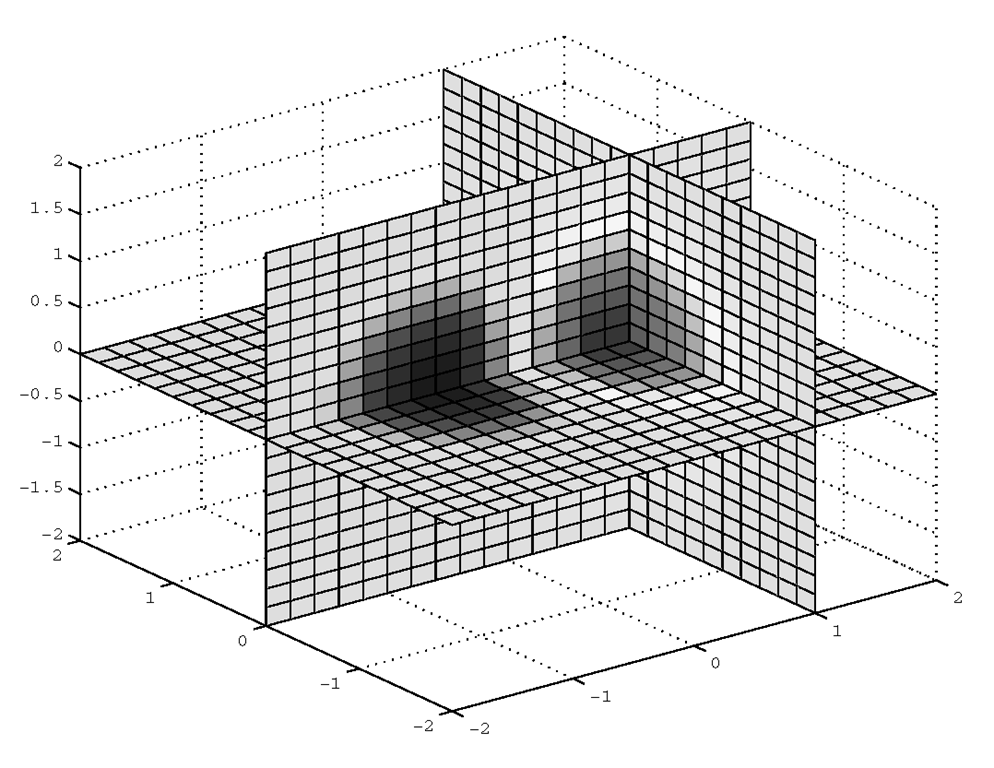
We can use the function slice to visualize slices through the volume, in this case at planes at x = 1, y = 0, and z = 0, as shown in Figure 4.38.

 

 

Figure 4.38 Slicing through a scalar volume.

MATLAB doesn’t limit you only to slices parallel to one of the axis planes. However, creating slice planes at arbitrary angles does require just a little bit of handle graphics. Here are the steps to slice with a plane at an arbitrary angle:

1. Create the surface to slice with by defining a surface and rotating it. You will need the handle to that surface in the following steps, so get it too. Here we use the bounds of the original volume as the bounds of our slice plane; notice how the z-axis is zeroed.

2. Rotate the slicing surface to the desired angle using the rotate function. Here we rotate only about the x-axis.

3. Use the get function to retrieve the data that defines the rotated slice plane.

4. Use slice to plot the new slice plane.

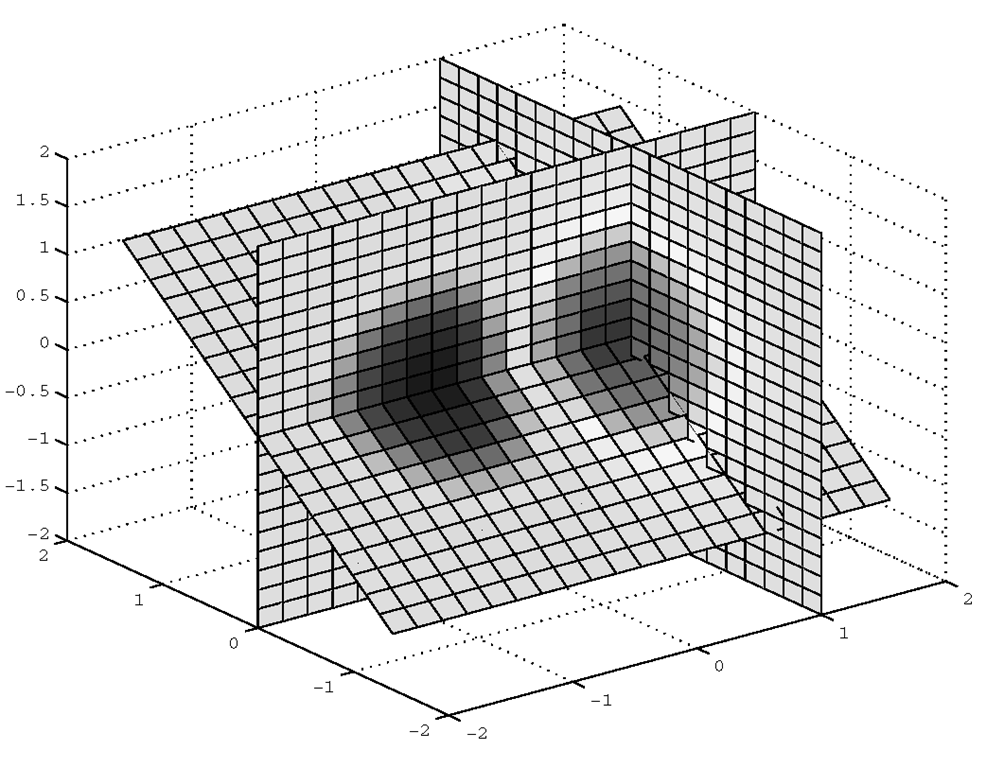
The result is shown in Figure 4.39.

Figure 4.39 A slice at -45 degrees.

Contour Slices

Contour lines can be added to slices readily with the function contourslice. This function is shown in its general form in Table 4.3.1b and as with other volume visualization functions, it takes the arrays defining the volume space (X, Y, and Z), and the value for the volume (V), but it also requires the slice plane specification (Sx, Sy, Sz). By default, contourslice will automatically assign contour line colors based on the value of the volume, but usually when we are combining slices with contours, we want our contour lines to be a single easy to see color and let the slice provide the color indicating the value of the volume. However, to do so requires the application of a little Handle Graphics, so without apology we present here the solution, as in the previous example. Let’s say we want to add white contour lines to the plot in Figure 4.39. This might seem a little challenging at first since our view includes both a vertical slice and then an intersecting slice at 45 degrees. Continuing with the previous example, here’s how to do it:

The first line plots 20 contour lines on the x = 1 plane and returns the handles to them.

For the 45-degree plane, we must be sure to use the slice plane data that defines that slice, i.e., xs, ys, and zs in this example.

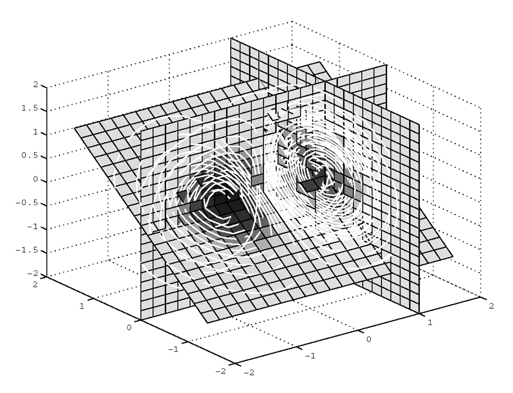
Figure 4.40 (see Plate 6) shows the result. Note that you do not have to have hold on with contourslice since it will hold the current plot itself.

Figure 4.40 Contour lines on slice planes.

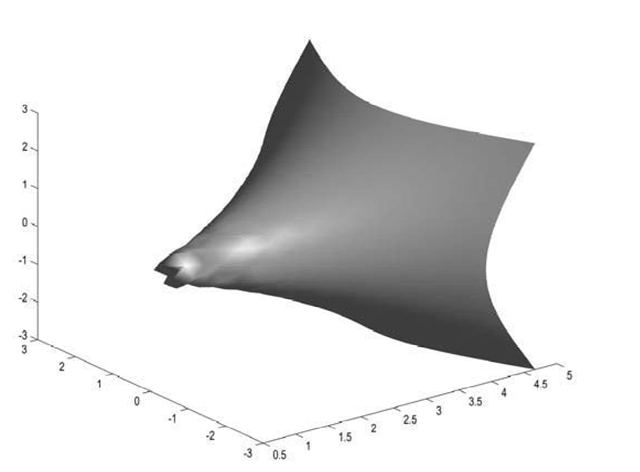
As a final note about slice planes, they don’t have to be planes at all! MATLAB allows you to use any surface you care to create in defining, what is more properly stated as, the slicing surface. To illustrate this, let’s continue with this same data, and slice it with the surface of a unit sphere.

First, put a slice in the original volume at x = 1. Be sure that hold on is activated.

Then get the surface definition for a sphere using MATLAB’s convenient sphere function. Recall that sphere will create a unit sphere centered at zero.

Now slice the volume with the sphere surface, and adjust the perspective with view for a better look.

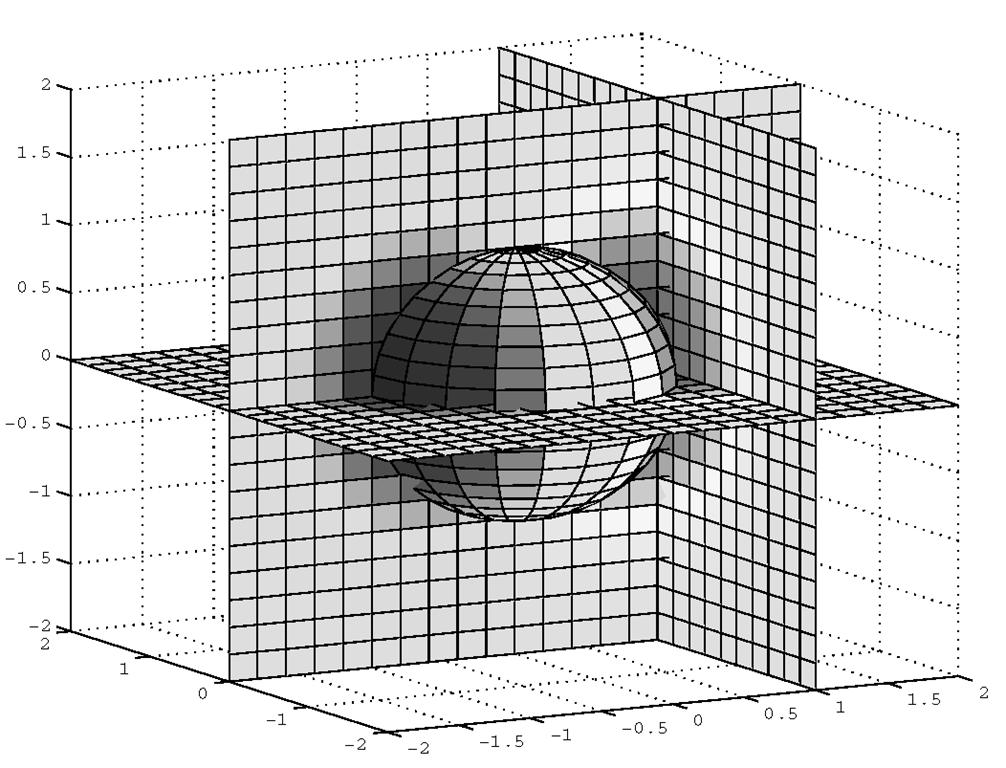
Your plot should look something like the one shown in Figure 4.41.

Figure 4.41 You can use any surface to "slice" a volume.

Isosurfaces and Isocaps

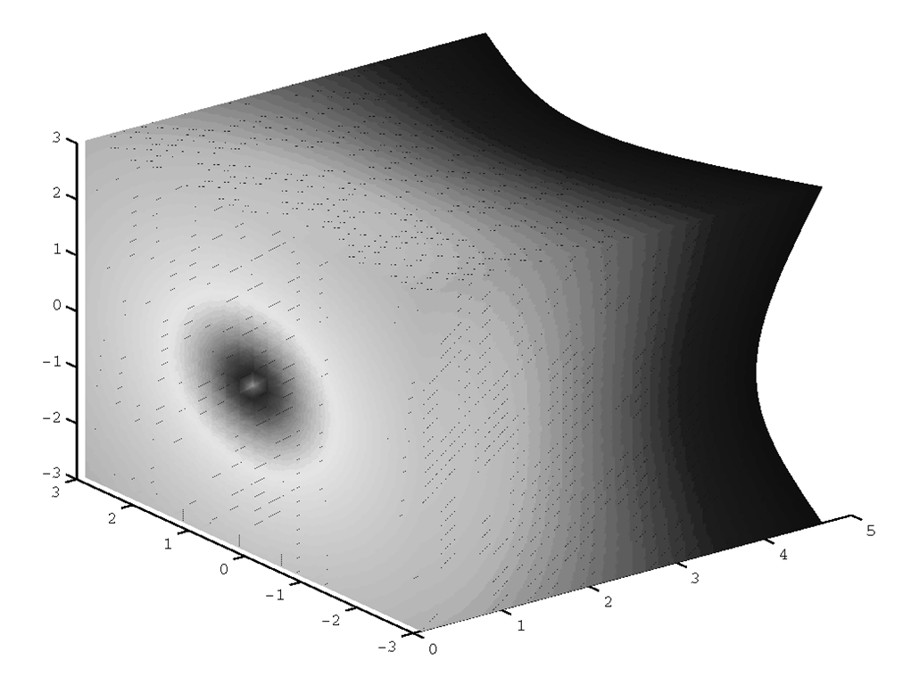
Another interesting and insightful method of volume visualization is to identify a surface throughout the space where the value of the volume is a constant. Just like contour lines connect values of z that are equal in a 2-D space where z=f(x,y), the function isosurface will outline in a volume where v=f(x,y,z) is a constant. To illustrate this, we will use a demonstration function included with MATLAB called flow. This is a function in three variables, and represents the speed profile of a submerged jet in an infinite tank. We like it because it produces an image with changing contours that readily illustrates interesting features of volume visualization. Let’s say we want to look at the flow data where it is equal to -1.5.

The resulting plot is shown in Figure 4.42.

Figure 4.42 An isosurface plot of the fluid function data at a value of -1.5.

Whereas isosurface outlines where a volume is of constant value, isocaps can be used to show what is inside the volume. Technically stated, isocaps computes an isosurface end-cap geometry for a given isovalue. Again, let’s consider the data generated by the flow function, but this time use isocaps.

The resulting visualization is shown in Figure 4.43.

Function	Action
[CURLX, CURLY, CURLZ, CAV] = curl(X,Y,Z,U,V,W)	Computes the curl and angular velocity (CAV) perpendicular to the flow of the 3-D vector field .
DIV = divergence(X,Y,Z,U,V,W)	Computes the divergence of the vector field.
VERTSOUT = interpstreamspeed(X,Y,Z,U,V,W,VERTICES)	Computes the streamline vertices (returning a cell array of vertex arrays) from vector field data U, V, and W, magnitudes (speed) by interpolation at vertices (such as those produced by stream2 or stream3) specified by the cell array VERTICES.

Table 4.3.2 Vector Volume Plotting Functions

Function	Action
XY = stream2(X,Y,U,V,STARTX,STARTY)	Computes 2-D stream line data, returning a cell array, XY, of vertex arrays suitable for use with plotting functions like streamline.
XYZ = stream3(X,Y,Z,U,V,W,STARTX,STARTY,STA RTZ)	Computes 3-D stream line data returning a cell array, XYZ, of vertex arrays suitable for use with plotting functions like streamline.
LIMS = volumebounds(X,Y,Z,U,V,W)	Returns the x- , y-, and z- axis coordinates and color limits for a volume as a vector LIMS = [xmin xmax ymin ymax zmin zmax cmin cmax].
[NX, NY, NZ, NV] = subvolume(X,Y,Z,V,LIMITS)	Extracts a subset of the volume data. The extent of the subset is specified in the vector LIMITS = [xmin, xmax, ymin, ymax, zmin, zmax], which contains coordinate values.
coneplot(X,Y,Z,U,V,W,Cx,Cy,Cz)	Plots velocity vectors as cones at the points Cx, Cy, and Cz in the vector field.
streamline(X,Y,Z,U,V,W,STARTX,STARTY,S TARTZ)	Draws stream lines from either 2D or 3-D vector data. STARTX, et al., define the starting positions of the stream lines.
streamparticles(VERTICES, N)	Draws stream particles using the vertices (such as those produced by stream2 or stream3) in the cell array VERTICES. N is the number of stream particles drawn, or the fraction of the total if less than 1. If not specified, the default is used, N=1, or 100% of the vertices.
streamribbon(X,Y,Z,U,V,W,STARTX,START	Draws stream ribbons from vector
Y,STARTZ)	data U, V, and W. STARTX, et al., define the starting positions of the stream lines at the center of the ribbons. The twist of the ribbons is proportional to the curl of the vector field.
streamslice(X,Y,Z,U,V,W,Sx,Sy,Sz)	Draws stream lines with direction arrows using the vector data U, V, and W, aligned in an x, y, z plane defined by Sx, Sy, Sz.
streamtube(X,Y,Z,U,V,W,STARTX, STARTY, STARTZ)	Draws stream tubes from vector data U, V, and W. STARTX, et al., define the starting positions of the stream lines at the center of the tubes.

Throughout this section on vector volume data, we will use an example data set included with MATLAB, wind.mat, that represents the air currents over North America. This data is made up of wind speed and direction vectors within a volume. You can access this data with the load command. Typing,load wind at the command prompt will load the data into the MATLAB workspace. (If you have been doing the examples as you read, you might want to first clear the workspace by issuing the clear command.) Once you load the wind data, you will have the volume arrays x, y, and z , and the volume vector arrays u, v, and w. We will use this data to illustrate the topics in this section.

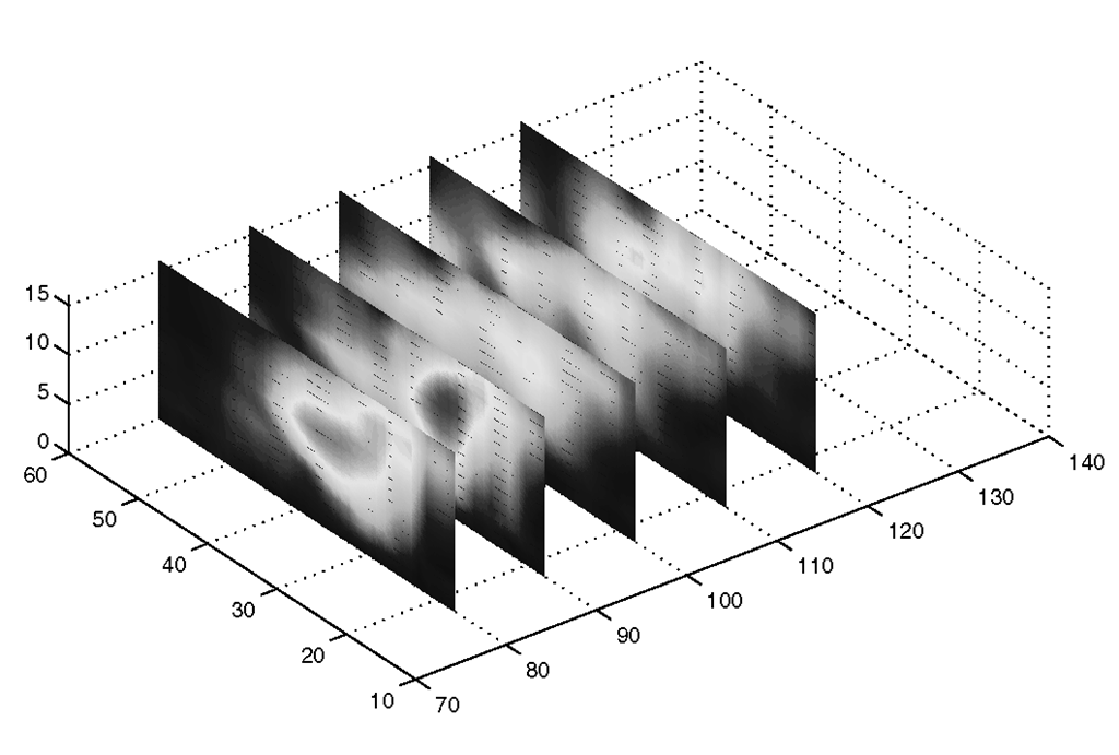
First, we must point out that although this section is concerned with volume data that has both magnitude and direction, you can still use scalar volume techniques with vector volume data; all you have to do is convert the vectors to scalars by computing the magnitude of the vectors. In the case of the wind data,

produces the plot shown in Figure 4.44.

Figure 4.44 Vector data plotted as scalar data.

However, Figure 4.44 gives us no information about the direction of the wind. In fact, we have lost that information completely in the computation of wind_vel. Now we shall turn our attention to stream plots, and how they are useful in visualizing the direction of flow within a volume.