These tools are just as applicable in the 3-D case as they are for 2-D plots. The Insert Text, Insert Arrow, etc., all work just as in the 2-D case; however be aware that if you annotate your plot before rotating it, the annotations will not move with the plot. This can lead to confusion and frustration so the rule of thumb is to set your view before you begin annotations. Simply select the cursor icon in the Figure Window toolbar to enter the plot edit mode, or type plotedit at the command prompt in the Command Window. Then, just as in the 2-D case, you can access each object in the figure and edit their properties by a simple point-and-click interface.
The Camera Toolbar
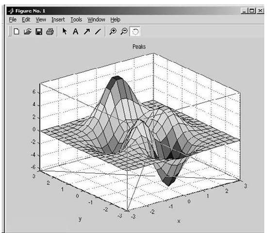
Here we will only deal with "simple" uses of the camera, namely those available from the Figure Window toolbar. To facilitate this discussion, open the Figure Window by creating a surface plot of the peaks function.
Now select View Camera Toolbar. When you do, the Camera Toolbar will appear in the Figure Window looking like Figure 4.33.
Figure 4.33 The Camera Toolbar in the Figure Window.
The Camera Motion Controls let you select different camera motion controls such as those that will orbit the camera or scene lighting, pan or tilt the camera, move the camera in and out, etc. The Principal Axis Selection tools provide a choice of axis about which some of the camera controls will operate. The Scene Lighting tool is a toggle that switches a light on or off. It can be useful in emphasizing the elevations and valleys in a surface. The Projection Type tool lets you choose between orthographic and perspective projections. Table 4.2.1 summarizes the two projection types, their consequences, and their use. The last two tool buttons, Reset Camera and Scene Light, and Stop Camera/Light Motion, let you reset the scene to the standard 3-D view and stop the camera from moving. In the next section, we will discuss the axis in general as it relates to 3-D graphics.
Table 4.2.1 Projection Types
|
Projection Type |
How to Interpret |
How to Use |
|
Orthographic Projection |
Think of the "viewing volume" as a box whose opposite sides are parallel, so the distance from the camera does not affect the size of surfaces in the plot |
Used to maintain the actual size of objects and the angle between objects. This works well for data plots. Real-world objects look unnatural. |
|
Perspective Projection |
The "viewing volume" is the projection of a pyramid where the apex has been cut off parallel to the base. Objects further from the camera appear smaller. |
Used to create more "realistic" views of objects. This works best for real-world objects. Data plots may look distorted. |
You can use the tools provided in the Figure Window to fine tune your plots, and it works well for single-use purposes, however the real power of MATLAB is in its programmability. Next, we will see how to manipulate the axis in code, as well as high-level color and shading manipulation.
Generalizing the Axis for 3 Dimensions
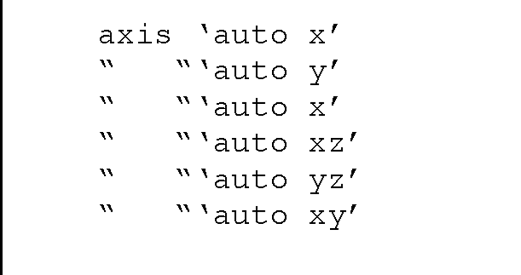
The axis function we used (axis([xmin xmax ymin ymax]) ) is fully generalized as axis([xmin xmax ymin ymax zmin zmax cmin cmax]), where xmin, ymin, and zmin are respectively the minimum x-, y-, and z-axis values, xmax, ymax, and zmax are the respective maximum x-, y-, and z-axis values, and cmin and cmax are color scaling limits. Uses such as axis(‘equal’), axis(‘ij’), and axis(‘xy’) also manipulate the 3-D plot but only the x- and y-axis of the current plot are affected.Table 4.2.2 summarizes the axis function syntax and its affect on a plot.
Table 4.2.2a Summary of the Axis Function
Table 4.2.2b Summary of the Axis Function
|
Syntax |
Affect |
|
axis equal |
Sets the aspect ratio of the x-, y-, and z-axis automatically according to the range of data units in the x, y, and z directions so that the data units are the same in every direction. This makes a sphere look like a sphere instead of an ellipsoid. |
|
axis image |
The same as axis(‘equal’) but also makes the plot box fit tightly around the data. |
|
axis square |
Adjusts the x-, y-, and z-axis so that they have equal lengths. This makes the axes region of 2-D plots square and of 3-D plots cubed. |
|
axis vis3d |
Freezes the aspect ratio so that rotation of 3-D objects will not "stretch-to-fi 11" the axes. |
|
axis normal |
Automatically adjusts the aspect ratio of the axes and data units on the axes to fill the plot. |
|
axis off or axis on |
Turns off or on all axis lines, tick marks, and labels. |
|
[mode,visibility,direc tion] = axis(‘state’) |
Returns the strings indicating the current axes settings: mode = ‘auto’ or ‘manual’ visibility = ‘on’ or ‘off direction = ‘xy’ or ‘ij’ |
3-D Plot Rotation
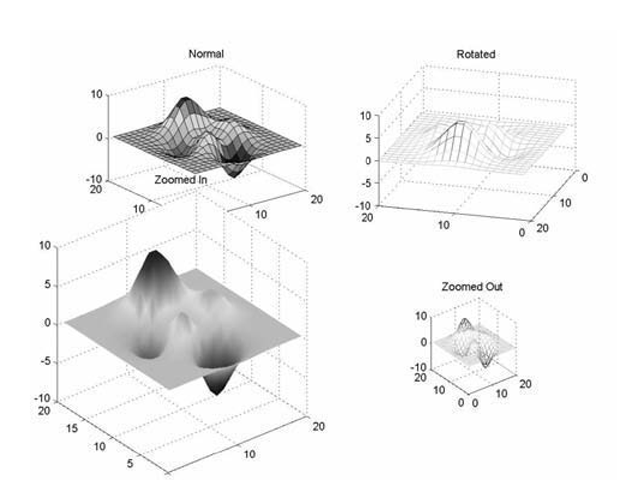
Recall the zooming and rotating buttons; these are still very much functional, and even more useful, with a 3-D plot. Figure 4.34 depicts the peaks function plotted differently in four subplots. Each subplot has been altered using either the zoom or rotate buttons. To zoom or rotate a subplot using the buttons, simply click on the button you wish to apply, then start clicking in the subplot. Notice that zooming changes the size of the axes by a factor of two in the subplot and can quickly overwhelm the other subplots.
Figure 4.34 The results of using the zooming and rotation tools from the Figure Window.
As you click on a plot to rotate it, if you hold the mouse button down you will see that MATLAB creates a reference box around the plot. You will also notice that the azimuth and elevation specifying the rotation is displayed in the Figure Window, but only as long as you keep the mouse button depressed. Figure 4.35 shows what you can expect to see.
Figure 4.35 The rotation box is visible while the mouse button is depressed.
The rotate tool can also be activated from the command line or M-File with rotate3d. In the next section we will discuss how to exercise greater control over our point-of-view of a 3-D plot.
Using the View Command
In the previous section, we saw how to use the rotation button to change the aspect, i.e., our point of view, of a 3-D plot. You noticed that as you kept the mouse button depressed, the Figure Window would indicate the aspect in terms of azimuth (Az) and elevation (El). You can achieve the same results from the command line or in your M-Files but with greater control by using the view function. The function view is used to specify the aspect you want to use to view a 3-D plot. You use it by calling it explicitly with two input arguments specifying the value of azimuth and elevation, or with a single input, being a vector with the values as its elements. When called with a two-element vector as an output argument, view will return the aspect currently in use.
In its simplest form, the function is used by passing an azimuth (Az) and elevation (El) angles in degrees as input arguments with view(Az,El) or with a single vector variable with two elements,view([Az El])
The angles are defined with respect to the axis origin, where the azimuth angle, Az, is in the xy-plane and the elevation angle, El, is relative to the x-y plane. Figure 4.36 depicts how to interpret the azimuth and elevation angles relative to the plot coordinate system.
Figure 4.36 The point-of-view in a 3-D plot.
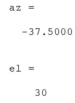
If you call view after creating a 3-D plot, it will return the current azimuth and elevation of the plot. If you have not previously changed these values, then this will return the default values of az = -37.5o and el = 30o. Consider again the surface plot of the peaks function.
The code,
will return
which are the default values for the azimuth and elevation.
As you have seen already, you can use the rotate tool from the Figure Window and change the aspect of the view of your plot. Let’s say that you have been merrily rotating away at your plot with the rotate tool, and now you have discovered that you can’t tell up from down in the figure. In such a situation, which happens more often than you might expect, view can come to your rescue. One way to use view is to issue the function with the default azimuth and elevation values.
However, even more convenient, the view function has two very simple forms that can help you when you get in such a bind. The forms of the function
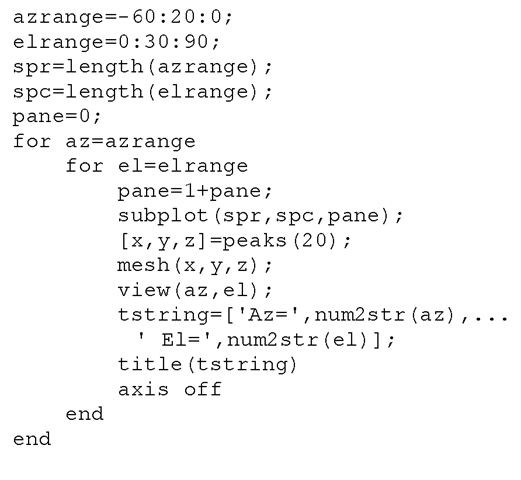
will restore the current plot to the default 3-D or 2-D views respectively. Again we visit the function peaks, this time presenting multiple views of it using the view function, as shown in Figure 4.37, created with the following code.
Figure 4.37 Multiple views of the peaks function.

