Simple 2-D Plot Manipulation (Plotting in Two Dimensions) (MATLAB) Part 3

Special Text Character Formats

You’ve seen that adding a string of text is relatively easy. You’ve even seen that you can have text in a title or on an axis label with more than one line by storing your strings in cell arrays. But in all these cases the text we provided were those characters available directly from our keyboard. What about special characters like the Greek alphabet, superscripts, subscripts, arrows, and other mathematical sysmbols?

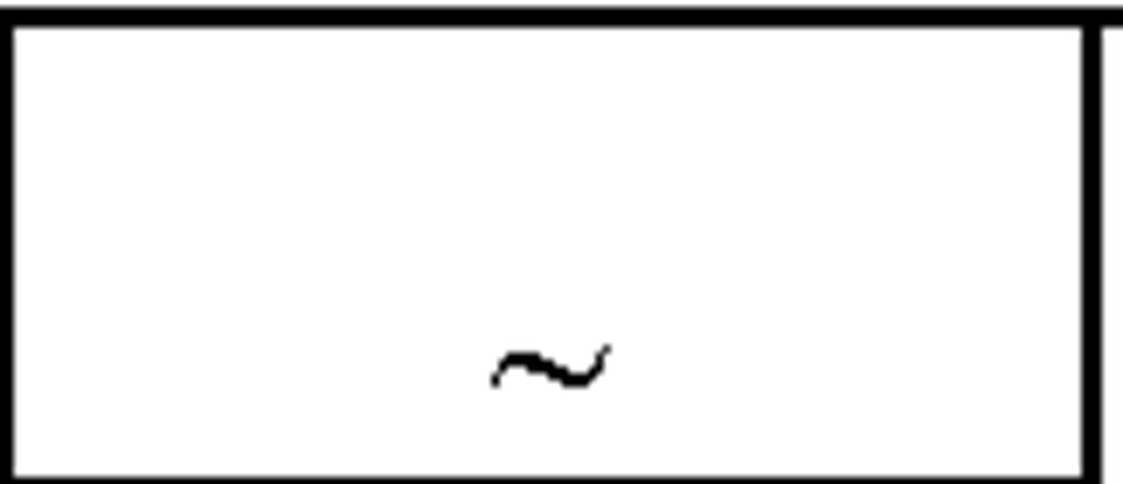
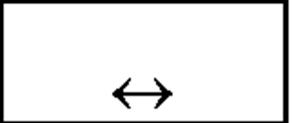
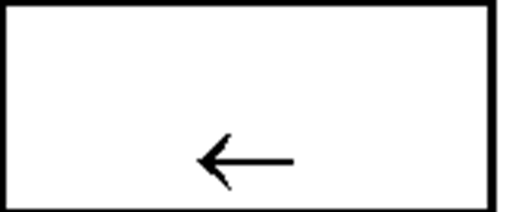
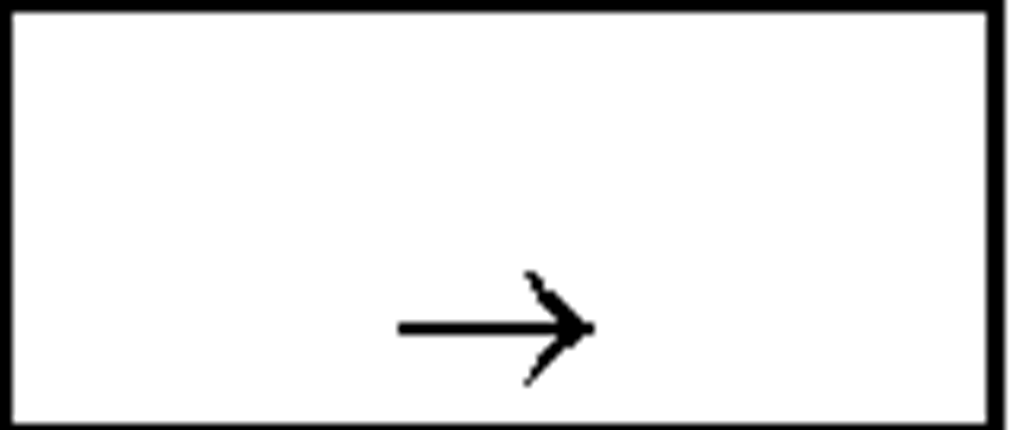
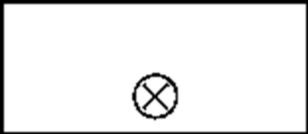
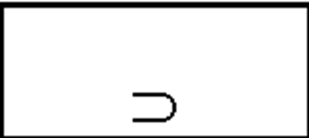
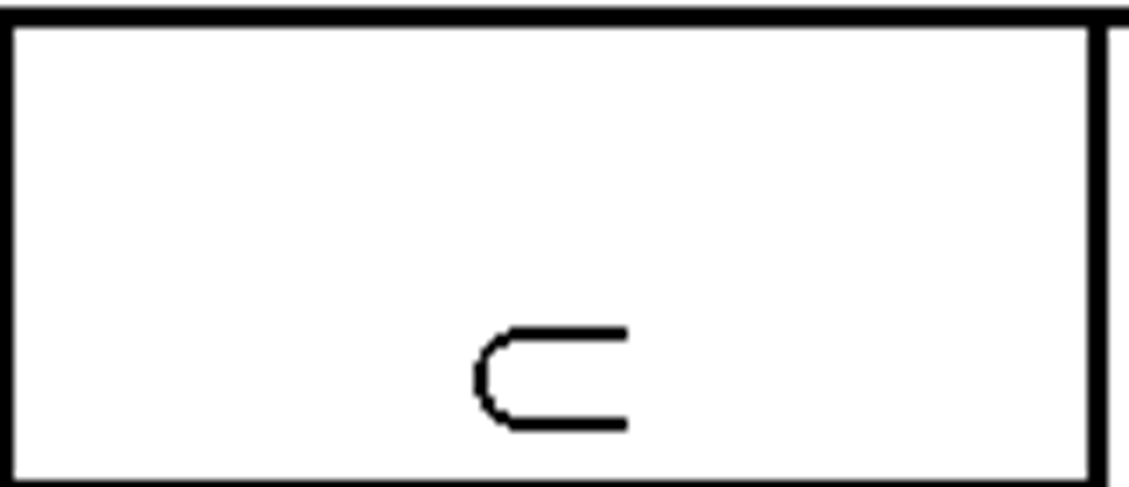
Fortunately MATLAB has the capability of modifying text to have different styles. It does this by providing support for a subset of the TeX characters. TeX is a standard notation for special character sets. You can recognize it right away as it will have a backslash "\" prefixing a character name. For example, the Greek character Ω (big omega) is specified by "\Omega" in TeX. Table 3.4.2 lists all the TeX characters available in MATLAB.

Table 3.4.2 TeX Characters Available in MATLAB

TeX Characters	Result	TeX Characters	Result	TeX Characters	Result
\alpha		\upsilon		\sim
\beta		\phi		\leq
\gamma		\chi		\infty
\delta		\psi		\clubsuit
\epsilon		\omega		\diamondsuit
\zeta		\Gamma		\heartsuit
\eta		\Delta		\spadesuit
\theta		\Theta		\leftrightarrow
\vartheta		\Lambda		\leftarrow
\iota		\Xi		\uparrow
\kappa		\Pi		\rightarrow
\lambda		\Sigma		\downarrow
\mu		\Upsilon		\circ
\nu		\Phi		\pm
\xi		\Psi		\geq
\pi		\Omega		\propto
\rho		\forall		\partial
\sigma		\exists		\bullet
\varsigma		\ni		\div
\tau		\cong		\neq
\equiv		\approx		\aleph
\Im		\Re		\wp
\otimes		\oplus		\oslash
\cap		\cup		\supseteq

TeX Characters	Result	TeX Characters	Result	TeX Characters	Result
\supset		\subseteq		\subset
\int		\in		\o
\rfloor		\lceil		\nabla
\lfloor		\cdot		\dots
\perp		\neg		\prime
\wedge		\times		\0
\rceil		\surd		\mid
\vee		\varpi		\copyright
\langle		\rangle

In addition to recognizing the special characters already listed, the MATLAB TeX interpreter also recognizes the following stream modifiers that control the font used.

Table 3.4.3 TeX Stream Modifiers

TeX Stream Modifier	Description
	Bold font.
	Italics font.
	Oblique font (rarely used).
	Normal font.
	Make part of string superscript.
	Make part of string subscript.
\fontname{fonfname}	Specify the font family to use.
\fontsize{fonfs/ze}	Specify the font size in FontUnits.

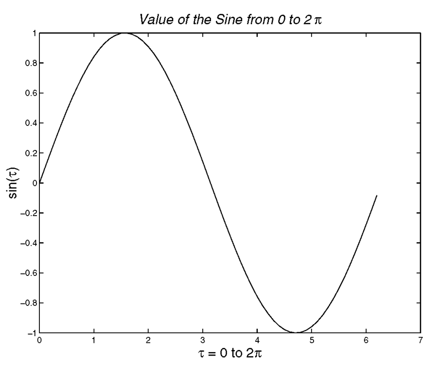
The first four modifiers are mutually exclusive so you can’t use them together. However, you can use \fontname in combination with one of the other modifiers. Also, stream modifiers remain in effect until the end of the string or only within the context defined by braces { }. The following code illustrates using the TeX interpreter and produces the plot shown in Figure 3.31.

 

 

 

Figure 3.31 Using TeX for special characters.

What about if you want to printSince    these    have meaning in the TeX interpreter you will need to tell the interpreter to ignore the command. This is achieved by using a backslash "\" right before them.

Using Subplot to Create Multiple Axes

You’ve seen that you can have multiple plots on an axis, either by plotting multiples or by using the hold command and issuing another plot command. However, you are not limited to having one axes object in a Figure Window. The easiest way to create multiple axes in a Figure Window is to make use of the command subplot. This function breaks up the Figure Window’s space into subregions or panes and is very useful for showing related information that is better viewed in individual plots. Calling the command with three arguments creates these subregions; the first two specify how many regions there will be in terms of rows and columns, and the third argument specifies which region you wish to plot in. For example, subplot(m,n,p) subdivides the Figure Window into m-by-n regions and creates axes in the pth region, where regions are numbered from left to right and top to bottom within the figure. For example, the following will break up the Figure Window into three distinct regions and create an axes object in the second one.

After you have created an axes object in one of the regions, you can then use any plotting command you want. The axes created with subplot can be treated in the same way as the ones that are created when no subregions are specified. In fact, you can create an axes object which encompasses the entire Figure Window’s space by issuing subplot(1,1,1) and get the same axes that you would have gotten by using plot commands without the subplot function.

If an axes already exists in the subregion identified with the subplot command, the existing axes becomes the current axes to which all subsequent graphics commands are issued. You can flip back and forth between these regions by re-issuing the subplot command to set one of the other axes or regions as the current axes.

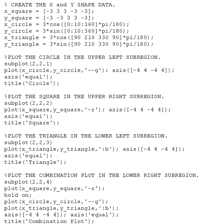
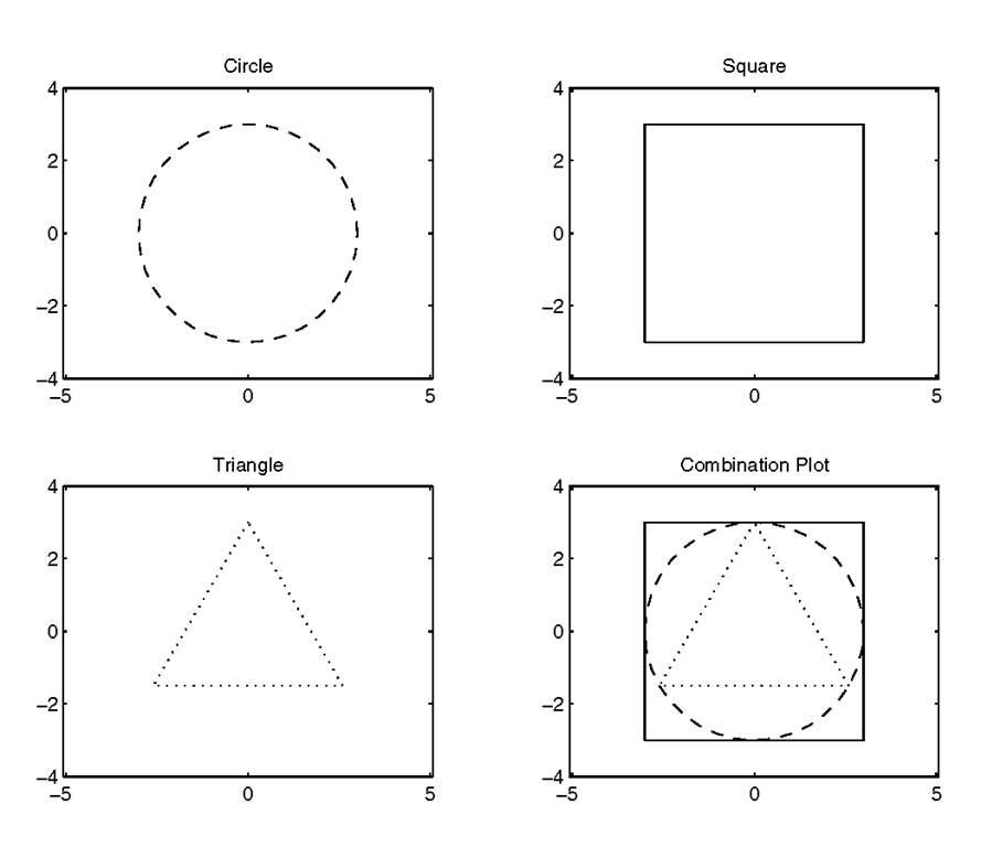
As an example, let’s break up the figure space into four panes configured in a 2-by-2 fashion. The following code will create a figure space with four subregions configured as a 2-by-2. We will plot three different shapes separately in the first three regions and then have the fourth subregion contain all three shapes superimposed on top of one another.

Figure 3.32 shows the results of this script.

Figure 3.32 Multiple axes with subplot.

Keep in mind, that if at any time you create a subplot that breaks up the figure into a new M-by-N configuration, the set of existing axes will be deleted!

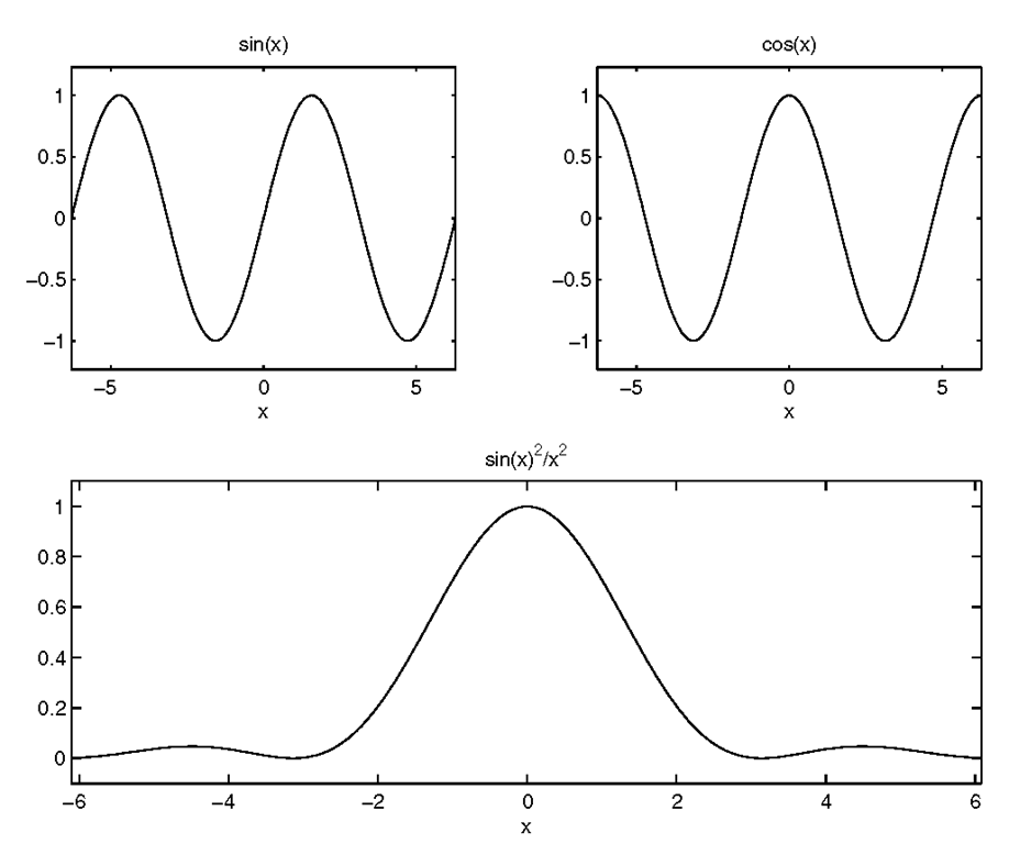
A useful (and undocumented) manipulation of the subplot can be used to place a different number of subplots on a row. For instance, instead of having four subplots in a two-by-two matrix, we could have two subplots on the top row and one subplot on the bottom row that spans the figure. The following code will create the plot shown in Figure 3.33.

The first two uses of subplot appear familiar enough; however, the final call specifies the large axis shown at the bottom of the figure. To create a similar figure with the single plot at the top use:

 

 

Figure 3.33 Odd axis made with subplot.

To create a subplot with one large plot axis on the left side and two small plot axes in a column on the right, use:

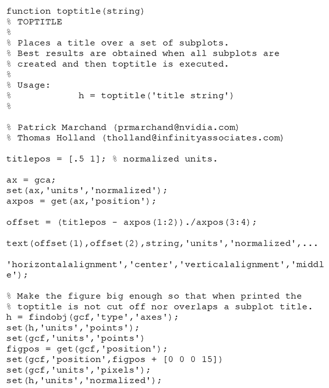
After you have created some subplots, you may have noticed that if you use the title command a title is created on top of the current axes. In some cases you may wish to have a title that is centered at the top of the Figure Window instead. Certainly you could use any of the text placement functions that were discussed previously such as gtext and text. However, if you do not want to be prompted or waited upon to place the text as with gtext, or you don’t want to determine the desired position’s relative location to the current axes as which would need to be done with text, you can use a function we include here called toptitle. This function will perform the calculations required to place a title string at the top of the figure regardless of the region to which you are currently plotting. The format for using toptitle is simply toptitle(string_vector) where string_vector is a character string containing the set of characters that you wish to have appear at the top of the figure.