We live in a three-dimensional world and much of our information is best revealed with 3-D techniques. Fortunately, MATLAB provides you with a cornucopia of graphics functions that let you make quick 3-D plots and visualizations of your data. This topic is intended to introduce you to these functions and lead you to a good understanding of the built-in MATLAB ability to visualize in three dimensions. We will begin by examining plot3, i.e., the three-dimensional counterpart to plot, and then examine the various surface creation techniques, followed by contour plots, and finally present MATLAB’s special functions for volume visualization.
Using Plot3
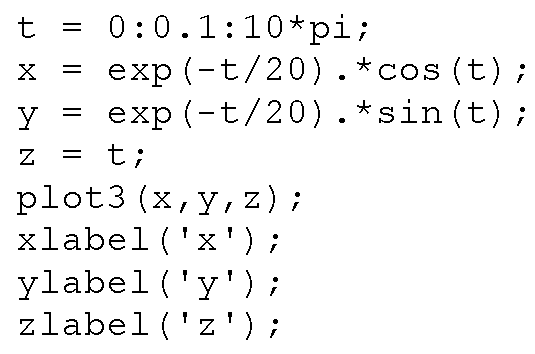
The plot3 function is used in almost the same way that plot is used, except that an additional variable, z, is used to provide the data for the third dimension. For example, let’s make use of the form plot3(x,y,z) by typing
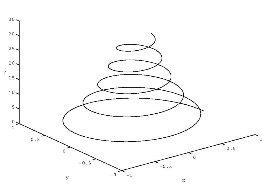
to produce Figure 4.1. Notice how the axes have been labeled using xlabel, ylabel, and here we introduce a new labeling command, zlabel, whose form is just like that of its siblings.
Figure 4.1 A 3-D plot using plot3.
The general form of this function is plot3(x, y, z, ‘string’), however what it does is determined by the nature of the variables passed to it, namely:
If x, y, and z are vectors of the same length, a 3-D line is created by connecting the coordinates specified by the elements of vectors x, y, and z.
If x, y, and z are matrices which have the same number of rows and columns, several lines will be created from the columns of the matrices.
If some of the input variables are matrices and others are vectors, and the vectors are the same length as either the number of rows or columns in the matrices, MATLAB will "replicate" the vectors in a fashion so that multiple lines can be created. If the sizes of the vectors or matrices do not permit this, MATLAB will return an error message.
The variable ‘string’ is a 1, 2, or 3 character string made from the characters compatible with the plot function (see Table 3.3.1).
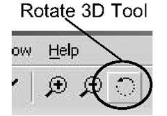
You can change the perspective, i.e., the viewing angle of plot by either one of two ways. First, you can select the Rotate 3-D tool from the Figure Window.
Doing so will let you to interactively rotate the axes of the plot by holding down the mouse button and moving the mouse about. The specific values of the azimuth and elevation will be shown in the lower left corner of the figure while you are rotating the axes.
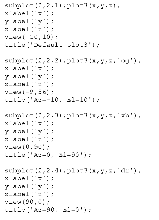
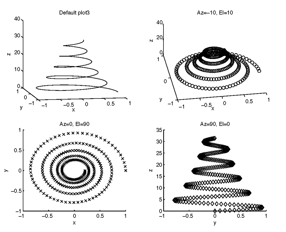
Your second option is to use the view function. The general form of this function is view(az, el) or view([az,el]) and with it you can specify the exact values of azimuth and elevation by which you wish to rotate the axes. The following code will produce the different views shown in Figure 4.2.
Figure 4.2 You can change your perspective by specifying az and el in the view function.
Although MATLAB’s native angle unit is radians, view uses degrees for the units of az and el. There are a few more interesting aspects of view that we will save for a later discussion, but for now you need to know that the default view for 3-D plots is az = -37.5° and el = 30o. Using az = 0o and el = 90o will give the default 2-D view; you can also obtain this by using view(2). What if you’ve rotated your axes so much that you are confused and you have grown tired of trying to fix it by dragging the mouse around? You can quickly return to the default 3-D view by typing view(3).
Creating 3-D Meshes and Surfaces
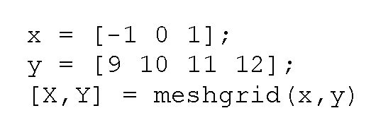
As we move into more 3-D plotting methods, we are going to find that often we must deal with ordered pairs, i.e., data that is dependent on both an x and a y value. Many mathematical functions are of two variables, that is, for each pair of x and y, there is a z. You have seen this stated as z = f(x,y). One way you could compute a z for each x y pair would be to iterate through a nested loop, but one of the major advantages of MATLAB is that it can deal with matrices without resorting to looping. All you need is some way to get your data into a matrix format. If you have a vector of x values, and a vector of y values, MATLAB provides a useful function called meshgrid that can be used to simplify the generation of X and Y matrix arrays used in 3-D plots. It is invoked using the form [X,Y] = meshgrid (x,y), where x and y are vectors that help specify the region in which coordinates, defined by element pairs of the matrices X and Y, will lie. The matrix X will contain replicated rows of the vector x, while Y will contain replicated columns of vector y. This might seem a little complicated at first, but an example will help make it clear. Consider the two vectors passed to meshgrid here.
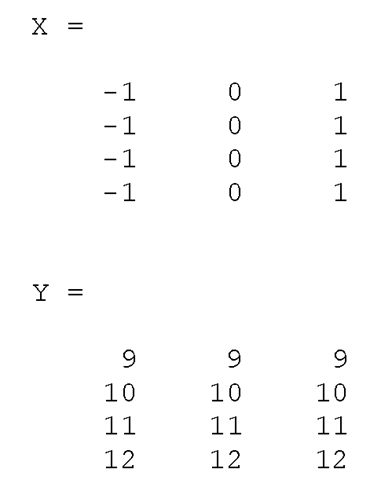
MATLAB returns
As you can see, X is formed by the vector x being replicated as rows for each column in y, and Y is formed by the vector y being replicated as columns for each element in x. Each element in x has been matched with each element in y. Be aware that typing meshgrid(x) is equivalent to meshgrid(x,x). The meshgrid function will be used in several of the examples in this section.
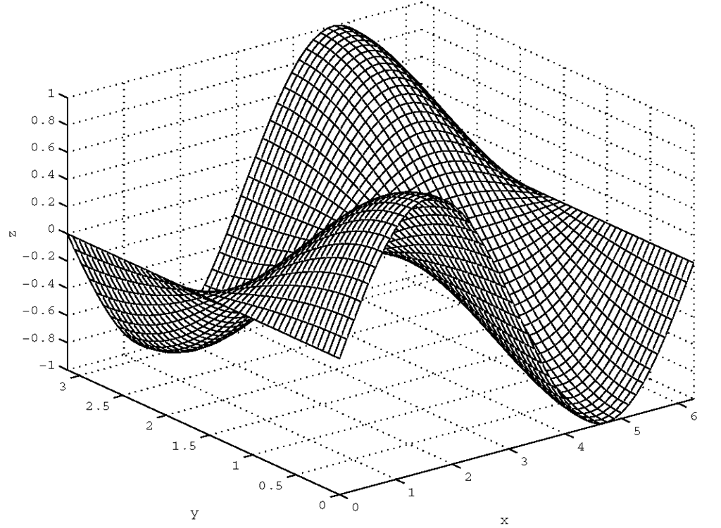
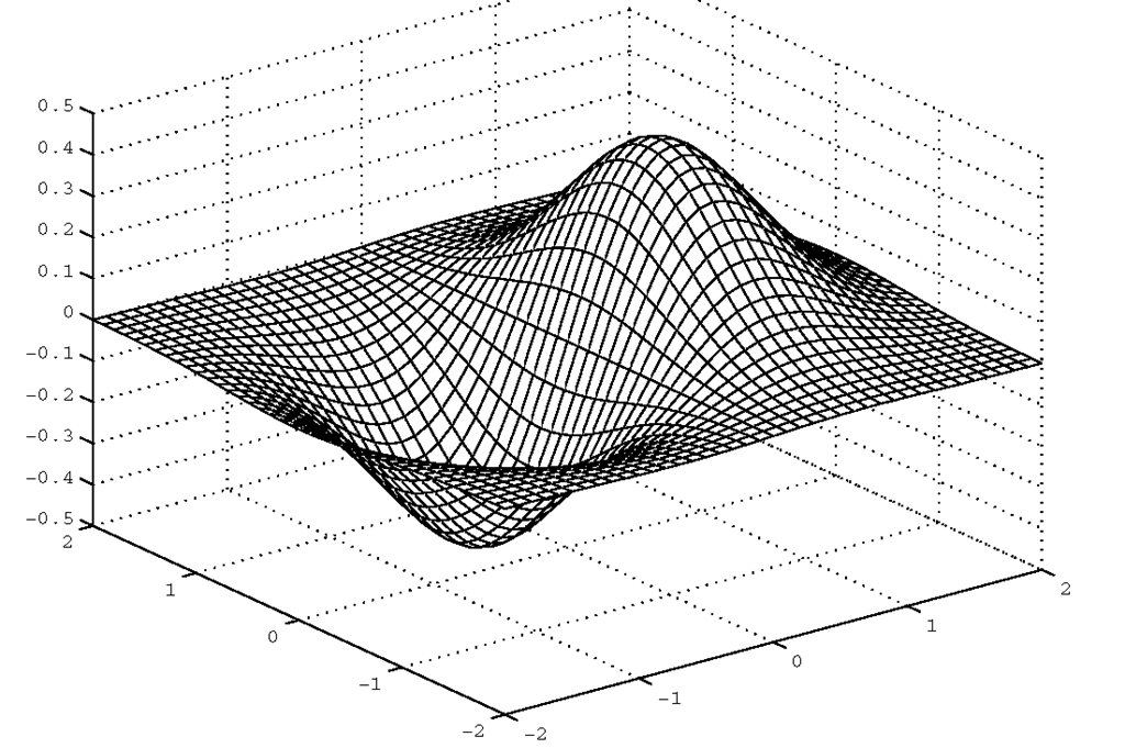
The first surface plotting function we will discuss is mesh. It creates many crisscrossed lines that look like a net draped over the surface defined by your data. To understand what the command is plotting, consider three M-by-N matrices, X, Y, and Z, that together specify coordinates of some surface in a three-dimensional space. A mesh plot of these matrices can be generated with the command mesh(X,Y,Z). Each (x(i,j),y(i,j),z(i,j)) triplet, corresponding to the element in the ith row and jth column of each of the X, Y, and Z matrices, is connected to the triplets defined by the elements in neighboring columns and rows. Vertices defined by triplets created from elements that are not in either an outer (i.e., first or last) row or column of the matrix will, therefore, be joined to four adjacent vertices. Vertices on the edge of the surface will be joined to three adjacent ones. Finally, vertices defining the corners of the surface will be joined only to the two adjacent ones. In addition to providing a visual perspective of the surface shape, this usage of mesh automatically chooses colors of the mesh plot to be proportional to the surface’s height. Consider the following example which will produce the plot shown in Figure 4.3 .
Figure 4.3 A simple mesh plot.
There are several ways to call the mesh command. We just looked at mesh(X,Y,Z), however, an even more general invocation of the function can be made with mesh(X,Y,Z,C) where the matrix C specifies the color of the mesh plot. When this C matrix is left out of the command, the function assumes that C = Z, thus providing a proportional mapping between color and surface height. For now it will suffice for you to realize that the minimum and maximum values of the matrix, C, specify the range of values that are associated with the figure’s color map, i.e., a list of RGB color vectors. The minimum value of C will be associated with the first row in the color map, and the maximum value of C will be associated with the last row in the color map. All values of C that lie between the minimum and maximum shall be associated with a color in this list. For example, if an element of C corresponding to one of the vertices lies halfway between the minimum and maximum values of C, the color associated with that vertex will lie halfway between the first and last row of the color map.Here is an example that demonstrates using manipulation of the color map to emphasize areas of identical slope. Consider the surface produced by,
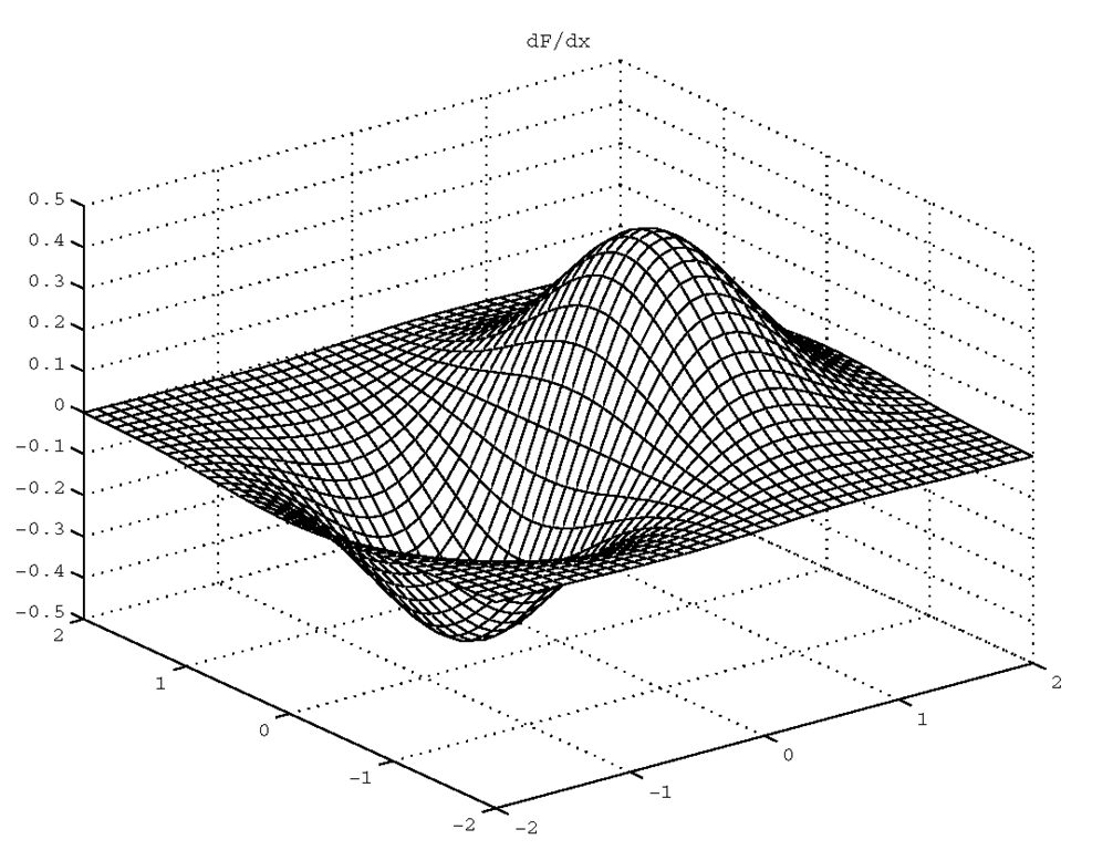
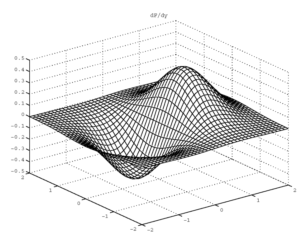
We can use mesh to plot this surface, however mesh will produce colors based on the values of z. We can use the gradient function to examine this surface and determine where the slopes are the same according to the x-axis and the y-axis. The general form is [Cx,Cy]=gradient(Z) where Cx is the numerically computed solution of ±Z/±x and Cy is ±Z/±y. (The actual gradient is the vector sum of Cx and Cy.) Since the derivative of function is its slope, the derivative taken at a point along the surface is the slope of the surface. By using the results of gradient as our color map, we can reveal those areas in the plot that have equal slope with respect to either the x, or y axes. The code that will show constant slope in the x-axis is,
The gradient function assumes an increment of 1, so we have specified it here to agree with our mesh. Figure 4.4 and Plate 1* shows the surface we are considering, plotted with mesh with its default coloring that varies according to the amplitude of z. Figure 4.5 and Plate 2 shows equal slopes with Cx from gradient. Figure 4.6 is the slope with respect to the y-axis dimension.
Figure 4.4 A default mesh plot with color assigned to height.
Figure 4.5 Identifying regions of slope with respect to the x-axis.
Figure 4.6 Identifying regions of slope with respect to the y-axis.
You should try this example on your computer so you can see the benefit of color better. Color, when used to actually convey information, can make a plot more informative and provides insight that may not have been achieved otherwise.
To finalize our discussion of the mesh function we need to mention that a mesh plot can also be created by passing two vectors, x and y, in place of the matrices, X and Y, by using either mesh(x,y,Z) or mesh(x,y,Z,C). The length vector x must be equal to the number of columns in Z, and the length of vector y must be equal to the number of rows in Z. When using this form of the command, a (x(j),y(i),Z(i,j)) triplet defines the vertices over the i rows and j columns of Z. If you do not provide the vectors x and y or matrices X and Y, to the function, e.g., when using mesh(Z) or mesh(Z,C), MATLAB creates a mesh plot by respectively setting the x and y vectors to the column and row number of the matrix Z.
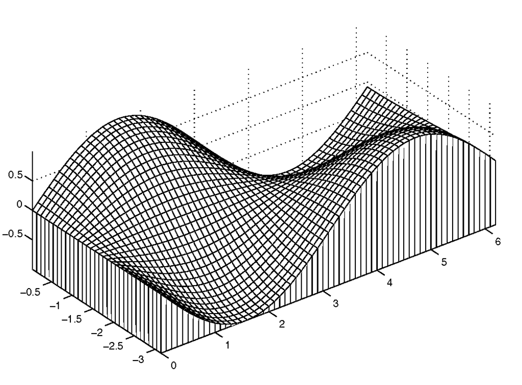
If you want to create a mesh plot that has a "curtain" around the edge of the surface, you might want to take advantage of the function meshz. This function is called with the identical input argument set used with mesh. The curtain is created by dropping lines down from the edge of the surface to a plane parallel to the xy-plane and at a height equal to the lowest point in the surface. For example,
will create the illustration shown in Figure 4.7.
Figure 4.7 A curtain mesh plot made with meshz.
