The parameterisation problems of the bias parameters in the GPS observation model are outlined in the Sect. 12.1 of the first edition of this topic. The problems are then mostly solved and the theory will be addressed here in detail.The equivalence properties of the algorithms of GPS data processing are described. The standard algorithms are outlined.
The commonly used GPS data processing methods are the so-called uncombined and combining, undifferenced and differencing algorithms (e.g., Hofmann-Wellenhof et al. 2001; Leick 2004; Remondi 1984; Seeber 1993; Strang and Borre 1997; Blewitt 1998). The observation equations of the combining and differencing methods can be obtained by carrying out linear transformations of the original (uncombined and undifferenced) equations. As soon as the weight matrix is similarly transformed according to the law of variance-cova-riance propagation, all methods are theoretically equivalent. The equivalences of combining and differencing algorithms are discussed in Sects. 6.7 and 6.8, respectively. The equivalence of the combining methods is an exact one, whereas the equivalence of the differencing algorithms is slightly different.The parameters are implicitly expressed in the discussions; therefore, the parameterisation problems of the equivalent methods have not been discussed in detail. At that time, this topic was considered one of the remaining GPS theoretical problems, and it will be discussed in the next subsection.
Three pieces of evidence of the parameterisation problem of the undifferenced GPS observation model are given first. Then the theoretical analysis and numerical derivation are made to show how to parameterise the bias effects of the undifferenced GPS observation model independently. A geometry-free illustration and a correlation analysis in the case of a phase-code combination are discussed. At the end, conclusions and comments are given.
Evidence of the Parameterisation Problem of the Undifferenced Observation Model
Evidence from Undifferenced and Differencing Algorithms
Suppose the undifferenced GPS observation equation and the related LS normal equation are
where all symbols have the same meanings as that of Eqs. 7.117 and 7.118. Equation 9.2 can be diagonalised as (cf. Sect. 7.6.1)
The related equivalent observation equation of the diagonal normal Eq. 9.3 can be written (cf. Sect. 7.6.1)
where all symbols have the same meanings as that of Eqs. 7.142 and 7.140. If X1 is the vector containing all clock errors, then the second equation of Eq. 9.3 is the equivalent double differencing GPS normal equation. It is well known that in a double differencing algorithm, the ambiguity sub-vector contained in X2 must be the double differencing ambiguities; otherwise, the problem will be generally singular. It is notable that X2 is identical with that of in the original undifferenced observation Eq. 9.1. Therefore, the ambiguity sub-vector contained in X2 (in Eq. 9.1) must be a set of double differencing ambiguities (or an equivalent set of ambiguities). This is the first piece of evidence (or indication) of the singularity of the undifferenced GPS observation model in which the undifferenced ambiguities are used.
Evidence from Uncombined and Combining Algorithms
Suppose the original GPS observation equation of one viewed satellite is (cf. Eq. 6.134)
then the uncombined or combining algorithms have the same solution of (cf. Eq. 6.138)
where all symbols have the same meanings as that of Eqs. 6.134 and 6.138. Then one notices that the ionosphere (£1) and geometry (Cp) are functions of the codes (R1 and R2) and are independent from phases![]() I in Eq. 9.6. In other words, the phase observables do not have any contribution to the ionosphere and geometry. And this is not possible. Such an illogical conclusion is caused by the parameterisation of the ambiguities given in the observation model of Eq. 9.5. If one takes the first evidence discussed above into account and defines that for each station one of the satellites in view must be selected as reference and the related ambiguity has to be merged into the clock parameter, then the phases do have contributions to ionosphere and geometry. One notices again that the parameterisation is a very important topic and has to be discussed more specifically. An improper parameterisation of the observation model will lead to incorrect conclusions through the derivation from the model.
I in Eq. 9.6. In other words, the phase observables do not have any contribution to the ionosphere and geometry. And this is not possible. Such an illogical conclusion is caused by the parameterisation of the ambiguities given in the observation model of Eq. 9.5. If one takes the first evidence discussed above into account and defines that for each station one of the satellites in view must be selected as reference and the related ambiguity has to be merged into the clock parameter, then the phases do have contributions to ionosphere and geometry. One notices again that the parameterisation is a very important topic and has to be discussed more specifically. An improper parameterisation of the observation model will lead to incorrect conclusions through the derivation from the model.
Evidence from Practice
Without using a priori information, a straightforward programming of the GPS data processing using an undifferenced algorithm leads to no results.Therefore an exact parameterisation description is necessary and will be discussed in the next section.
A Method of Uncorrelated Bias Parameterisation
We restrict ourselves here to discuss the parameterisation problem of the bias parameters (or constant effects, i.e., the clock errors and ambiguities) only.
Recall the discussions of the equivalence of undifferenced and differencing algorithms in Sect. 6.8. The equivalence property is valid under three conditions: observation vector L used in Eq. 9.1 is identical; parameterisation of X2 is identical; and X1 is able to be eliminated (cf. Sect. 6.8).
The first condition is necessary for the exactness of the equivalence because of the fact that through forming differences, the unpaired data will be cancelled out in the differencing.
The second condition states that the parameterisation of the undifferenced and differencing model should be the same. This may be interpreted as the following: the rank of the undifferenced and differencing equations should be the same if the differencing is formed by a full rank linear transformation. If only the differencing equations are taken into account, then the rank of the undifferenced model should equal the rank of the differencing model plus the number of eliminated independent parameters.
It is well known that one of the clock error parameters is linearly correlated with the others. This may be seen in the proof of the equivalence property of the double differences, where the two receiver clock errors of the baseline may not be separated from each other and have to be transformed to one parameter and then eliminated.This indicates that if in the undifferenced model all clock errors are modelled, the problem will be singular (i.e. rank defect). Indeed, Wells et al. (1987) noticed that the equivalence is valid if measures are taken to avoid rank defect in the bias parameterisation. Which clock error has to be kept fixed is arbitrary. Because of the different qualities of the satellite and receiver clocks, a good choice is to fix a satellite clock error (the clock is called a reference clock). In practice, the clock error is an unknown; therefore, there is no way to keep that fixed except to fix it to zero. In such a case, the meaning of the other bias parameters will be changed and may represent the relative errors between the other biases.
The third condition is important to ensure a full-ranked parameterisation of the parameter vector X1, which is going to be eliminated.
The undifferenced Eq. 9.1 is solvable if the parameters X1 and X2 are not over-parameterised. In the case of single differences, X1 includes satellite clock errors and is able to be eliminated. Therefore, to guarantee that the undifferenced model Eq. 9.1 is not singular, X2 in Eq. 9.1 must be not over-parameterised. In the case of double differences, X1 includes all clock errors except the reference one. Here we notice that the second observation equation of 9.1 is equivalent to the double differencing observation equation and the second equation of 9.2 is the related normal equation. In a traditional double differencing observation equation, the ambiguity parameters are represented by double differencing ambiguities. Recall that for the equivalence property, the number (or rank) of ambiguity parameters in X2 that are not linearly correlated must be equal to the number of the double differencing ambiguities. In the case of triple differences, X1 includes all clock errors and ambiguities. The fact that Xj should able to be eliminated leads again to the conclusion that the ambiguities should be linearly independent.
The two equivalent linear equations should have the same rank. Therefore, if all clock errors except the reference one are modelled, the number of independent undifferenced ambiguity parameters should be equal to the number of double differencing ambiguities. According to the definition of the double differencing ambiguity, one has for one baseline
where i1 and i2 are station indices, kj is the jth satellite’s identification, n is the common observed satellite number and is a function of the baseline, and N is ambiguity. Then there are n- 1 double differencing ambiguities and 2n undifferenced ambiguities. Taking the connection of the baselines into account, there are n- 1 double differencing ambiguities and n new undifferenced ambiguities for any further baseline. If i1 is defined as the reference station of the whole network and k1 as the reference satellite of station i2, then undifferenced ambiguities of the reference station cannot be separated from the others (i.e., they are linearly correlated with the others). The undifferenced ambiguity of the reference satellite of station i2 cannot be separated from the others (i.e., it is linearly correlated with the others). That is, the ambiguities of the reference station cannot be determined, and the ambiguities of the reference satellites of non-reference stations cannot be determined. Either they should not be modelled or they should be kept fixed. A straightforward parameterisation of all undifferenced ambiguities will lead to rank defect, and the problem will be singular and not able to be solved.
Therefore, using the equivalence properties of the equivalent equation of GPS data processing, we come to the conclusion that the ambiguities of the reference station and ambiguities of the reference satellite of every station are linearly correlated with the other ambiguities and clock error parameters. However, a general method of parameterisation should be independent of the selection of the references (station and satellite). Therefore, we use a two-baseline network to further our analysis. The original observation equation can be written as follows:
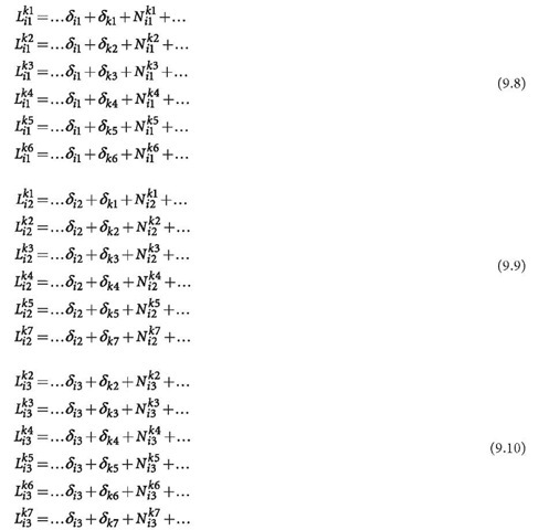
where only the bias terms are listed and L and 8 represent observable and clock error, respectively. Observation equations of station i1, i2 and i3 are Eqs. 9.8, 9.9 and 9.10. Define that the baseline 1, 2 are formed by station i1 and i2, as well as i2 and i3, respectively. Select i1 as the reference station and then keep the related ambiguities fixed (set to zero for simplification). For convenience of later discussion, select![]() as the reference clock (set to zero, too) and select
as the reference clock (set to zero, too) and select![]() as reference satellites of the station i2, i3 (set the related ambiguities to zero), respectively. Then Eqs. 9.8-9.10 become
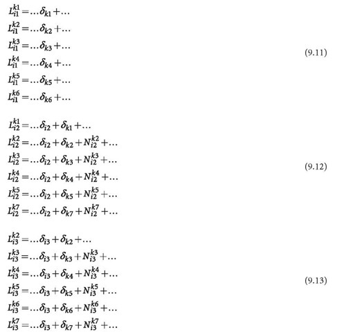
as reference satellites of the station i2, i3 (set the related ambiguities to zero), respectively. Then Eqs. 9.8-9.10 become
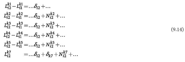
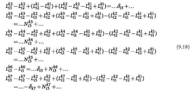
Differences can be formed through linear operations. The total operation is a full rank linear transformation, which does not change the least squares solution of the original equations. Single differences can be formed by the following (Eq. 9.11 remains unchanged and therefore will not be listed again):
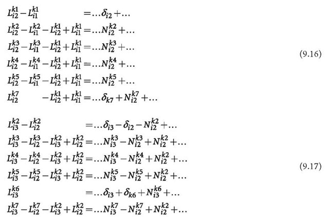
where two observations are unpaired due to the baseline definitions. Double differences can be formed by
Using Eqs. 9.16 and 9.11, Eq. 9.17 can be further modified to
or
From the last equation of Eqs. 9.16 and 9.19, it is obvious that the clock error and the ambiguities of satellite k7, which is not observed by the reference station, are linearly correlated. Keeping one of the ambiguities of the satellite k7 at station i2 or i3 is necessary and equivalent. Therefore, for any satellite that is not observed by the reference station, one of the related ambiguities should be kept fixed (station selection is arbitrary). In other words, one of the ambiguities of all satellites has to be kept fixed. In this way, every transformed equation includes only one bias parameter and the bias parameters are linearly independent (regular). Furthermore, the differencing cannot be formed for the unpaired observations of every baseline. However, in the case of an undifferenced adjustment, the situation would be different. We notice that the equation for k6 in Eq. 9.18 can be transformed to a double differencing one in Eq. 9.19. If more data is used in the undifferenced algorithm than in the differencing method, the number of undifferenced ambiguity parameters will be larger than that of the double differencing ones. Therefore, we have to drive the so-called data condition to guarantee that the data are able to be differenced, or equivalently, we have to extend the way of double differencing forming so that the differencing will be not limited by special baseline design. Both will be discussed in Sect. 9.2.
The meanings of the parameters are changed by independent parameterisation, and they can be read from Eqs. 9.11-9.13. The clock errors of the satellites observed by the reference station include the errors of receiver clock and ambiguities. The receiver clock errors include the error of ambiguity of the reference satellite of the same station. Due to the inseparable property of the bias parameters, the clock error parameters no longer represent pure clock errors, and the ambiguities represent no longer pure physical ambiguity. Theoretically speaking, the synchronisation applications of GPS may not be realised using the carrier-phase observations. Furthermore, Eq. 9.19 shows that the undifferenced ambiguities of i3 have the meaning of double differencing ambiguities of the station i3 and i1 in this case.
Up to now, we have discussed the correlation problem of the bias parameters and found a method of how to parameterise the GPS observations regularly to avoid the problem of rank defect. Of course, many other ways to parameterise the GPS observation model can be similarly derived. However, the parameter sets should be equivalent to each other and can be transformed from one set to another uniquely as long as the same data is used.
Geometry-Free Illustration
The reason why the reference parameters have to be fixed lies in the nature of range measurements, which cannot provide information of the datum origin (cf., e.g., Wells et al. 1987, p 9). Suppose d is the direct measurement of clock errors of satellite k and receiver i, i.e.![]() no matter how many observations were made and how the
no matter how many observations were made and how the
indices were changed, one parameter (i.e. reference clock) is inseparable from the others and has to be fixed. Suppose h is the direct measurement of ambiguity Nand clock errors of satellite k and receiver i, i.e.,![]() the number of over-parameterised biases is exactly the number of total observed satellites and used receivers. This ensures again that our parameterisation method to fix the reference clock and one ambiguity of every satellite as well as one ambiguity of the reference satellite of every non-reference station is reasonable. The case of combination of d and h (as code and phase observations) will be discussed in the next section.
the number of over-parameterised biases is exactly the number of total observed satellites and used receivers. This ensures again that our parameterisation method to fix the reference clock and one ambiguity of every satellite as well as one ambiguity of the reference satellite of every non-reference station is reasonable. The case of combination of d and h (as code and phase observations) will be discussed in the next section.
Correlation Analysis in the Case of Phase-Code Combinations
A phase-code combined observation equation can be written by (cf. Sect. 7.5.2)
where![]() are the observational vectors of phase (scaled in length) and code, respectively;
are the observational vectors of phase (scaled in length) and code, respectively;![]() are related residual vectors;
are related residual vectors;![]() are unknown vectors of ambiguity and others;
are unknown vectors of ambiguity and others;![]() are related coefficient matrices;
are related coefficient matrices;![]() is a symmetric and definite weight matrix; and
is a symmetric and definite weight matrix; and![]() are weight factors of the phase and code observations.
are weight factors of the phase and code observations.
The phase, code and phase-code normal equations can be formed respectively by
where
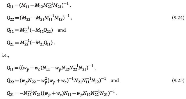
The covariance matrix Q is denoted
where (Gotthardt 1978; Cui et al. 1982)
Thus the correlation coefficient![]() is a function of
is a function of![]()
where indices i and j are the indices of unknown parameters in![]() (only phase is used,
(only phase is used,![]() _ are partly linear correlated) and
_ are partly linear correlated) and![]() are uncorrelated), there exists indices ij, so that
are uncorrelated), there exists indices ij, so that
In other words, there exists indices i and j, the related unknowns are correlated if ![]() and uncorrelated if
and uncorrelated if![]() In the case of a phase-code combination,
In the case of a phase-code combination,![]() can be selected, and one has
can be selected, and one has
whose value should be very close to 1 (strong correlated) in the discussed case. Equations 9.26, 9.27 and 9.28 indicate that for the correlated unknown pair ij, the correlation situation may not change much by combining the code to the phase because of the lower weight of the code related to the phase. A numerical test confirmed this conclusion.
Conclusions and Comments
In this section, the singularity problem of the undifferenced GPS data processing is pointed out and an independent parameterisation method is proposed for bias parameters of the GPS observation model. The method is implemented into software, and the results confirm the correctness of the theory and algorithm. Conclusions can be summarised by
1. Bias parameterisation of undifferenced GPS phase observations with all clock errors except the reference one, and all undifferenced ambiguities are linearly correlated. The linear equation system of undifferenced GPS is then singular and cannot be solved theoretically;
2. A linear independent bias parameterisation can be reached by fixing the reference clock of the reference station, fixing one of the ambiguities of every satellite of arbitrary station (called reference station of every satellite), and fixing the ambiguities of the reference satellite of every non-reference station. The selections of the references are arbitrary; however, the selections are not allowed to be duplicated;
3. The linear independent ambiguity parameter set is equivalent to the parameter set of double differencing ambiguities, and they can be transformed from one to another uniquely if the same data is used;
4. The physical meanings of the bias parameters are varied depending on the way of parameterisation. Due to the inseparable property of the bias parameters, the synchronisation applications of GPS may not be realised using the carrier-phase observations;
5. The phase-code combination does not change the correlation relation between the correlated biases significantly.
Due to the facts regarding the use of the undifferenced algorithm, it is worthy to give some comments:
1. In the undifferenced algorithm, the observation equation is a rank defect one if the over-parameterisation problem has not been taken into account. The numerical inexactness introduced by eliminating the clock error parameters and the use of a priori information of some other parameters are the reason why the singular problem is solvable in practice so far;
2. Using the undifferenced and differencing methods, solutions of the common parameters must be the same if the undifferenced GPS data modelling is really an equivalent one and not over-parameterised;
3. A singular undifferenced parameterisation may become regular by introducing conditions or by fixing some of the parameters through introducing a priori information.


