As discussed in Sect. 8.3.7, a normal equation can be diagonalised and the related observation equation can be formed.
For the linearised observation equation (cf. Eq. 8.38)
the least squares normal equation can be written as (cf. Eqs. 8.39 and 8.40)
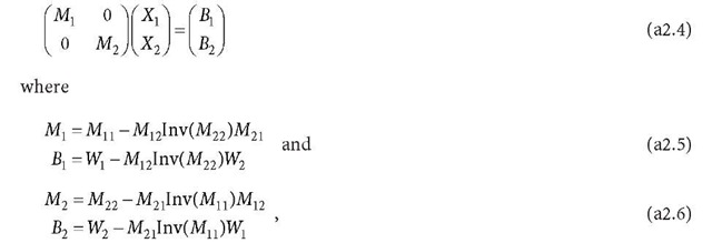
The normal Eq. a2.2 can be diagonalised as (cf. Eq. 8.41)
The above diagonalisation process can be repeated r – 1 times to the second normal equation of Eq. a2.4, so that the second equation of Eq. a2.4 can be fully diagonalised and Eq. a2.4 can be represented as:
where![]() is a diagonal matrix, r is the dimension of
is a diagonal matrix, r is the dimension of![]() is a vector.
is a vector.
Normal Eq. a2.4 related observation equation is (cf. Eq. 8.43)
where E is an identity matrix, and![]() are residual vectors, which have the same property as V in Eq. a2.1.
are residual vectors, which have the same property as V in Eq. a2.1.
By similarly repeating the above process r – 1 times to the observation equation of X2 (i.e., the second equation of Eq. a2.8), then Eq. a2.8 turns out to have a form of
where![]() is in a form of a diagonal matrix where all elements are vectors of dimension r, P is a diagonal matrix of P,L’is a vector of L, and 1*2 is a residual vector that has the same property as V in Eq. a2.1. Equation a2.11 is the observation equation of normal Eq. a2.7.
is in a form of a diagonal matrix where all elements are vectors of dimension r, P is a diagonal matrix of P,L’is a vector of L, and 1*2 is a residual vector that has the same property as V in Eq. a2.1. Equation a2.11 is the observation equation of normal Eq. a2.7.
Numerical examples to illustrate the diagonalisation process of the normal equation and observation equation are given below.
1. The Case of Two Variables
For the observation equation (where o is set to 1, which does not affect all results)
the least squares normal equation is
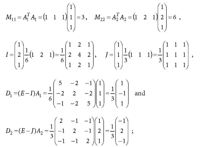
Because
Eq. a2.13 is diagonalised as
The solution![]() of Eq. a2.14 is the same as that of Eq. a2.13. Furthermore, to form the equivalent observation equation, there are
of Eq. a2.14 is the same as that of Eq. a2.13. Furthermore, to form the equivalent observation equation, there are
thus, the observation equation related to Eq. a2.14 is
The normal equation of the observation Eq. a2.15 is exactly the same as Eq. a2.14. This numerical example shows that the normal equation and the related observation equation can be diagonalised.
2. The Case of Three Variables
For the observation equation (where o is set to 1, which does not affect all results)
the least squares normal equation is
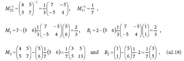
Because
Eq. a2.17 is diagonalised as
The![]() related normal equation can be further diagonalised. Because of
related normal equation can be further diagonalised. Because of
Eq. a2.19 is further diagonalised as
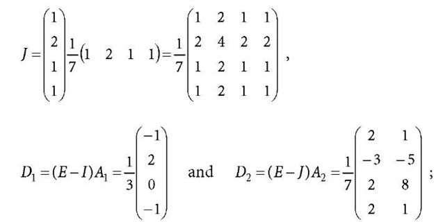
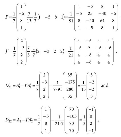
The solution![]() of Eq. a2.20 is the same as that of Eqs. a2.17 and a2.19. Furthermore, to form the equivalent observation equation of Eq. a2.19, there are
of Eq. a2.20 is the same as that of Eqs. a2.17 and a2.19. Furthermore, to form the equivalent observation equation of Eq. a2.19, there are
thus, the observation equation related to Eq. a2.19 is
The X2 and X3 related observation equation can be further diagonalised as follows. Because
the observation equation related to Eq. a2.20 is
The normal Eq. a2.17 and its related observation Eq. a2.16 are fully diagonalised as Eqs. a2.20 and a2.22, respectively. These numerical examples show that the normal equation and the related observation equation can be diagonalised as described in Sect. 8.3.7.


