For any linear equation system
a linear transformation can be defined as a multiplying operation of matrix T to Eq. 6.39, i.e.,
where T is called the linear transformation matrix and has a dimension of k x m. An inverse transformation of T is denoted by![]() An invertible linear transformation does not change the property (and solutions) of the original linear equations. This may be verified by multiplying
An invertible linear transformation does not change the property (and solutions) of the original linear equations. This may be verified by multiplying![]() to Eq. 6.40. A non-invertible linear transformation is called a rank deficient (or not full rank) transformation.
to Eq. 6.40. A non-invertible linear transformation is called a rank deficient (or not full rank) transformation.
The covariance matrix of L is denoted by cov(L) or QLL (cf. Sect. 6.2); then the co-variance of the transformed L (i.e., TL) can be obtained by covariance propagation theorem by (cf., e.g., Koch 1988)
where superscript T denotes the transpose of the transformation matrix.
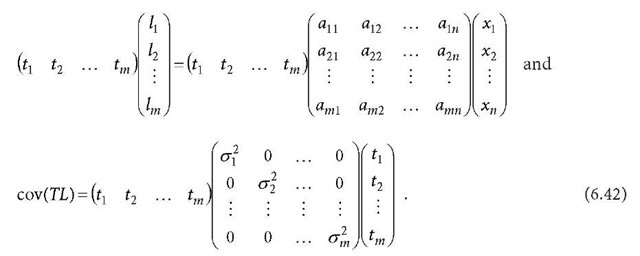
If transformation matrix T is a vector (i.e., k =1) and L is an inhomogeneous and independent observable vector (i.e., covariance matrix![]() is a diagonal matrix with elements of
is a diagonal matrix with elements of![]() is the variance (
is the variance (![]() is called standard deviation) of the observable lj), then Eqs. 6.40 and 6.41 can be written as
is called standard deviation) of the observable lj), then Eqs. 6.40 and 6.41 can be written as
Equation 6.43 is called the error propagation theorem. 6.5


