Data differentiations are methods of combining GPS data (of the same type) measured at different stations. For the convenience of later discussions, tidal effects and relativ-istic effects are considered corrected before forming the differences. The original code, phase and Doppler observables as well as their standardised combinations can be rewritten as (cf. Eqs. 6.44-6.47)
where![]() is the index of frequency f, subscript i is the index of station number and superscript k is the id number of satellite.
is the index of frequency f, subscript i is the index of station number and superscript k is the id number of satellite.
Single Differences
Single difference (SD) is the difference formed by data observed at two stations on the same satellite as
where O is the original observable, and![]() are two id number of the stations.
are two id number of the stations.
Supposing the original observables have the same variance of![]() then the single difference observable has a variance of
then the single difference observable has a variance of![]() Considering Eqs. 6.89-6.92, one has
Considering Eqs. 6.89-6.92, one has
where![]() is the time differentiation of
is the time differentiation of![]() are the differenced ionospheric and tropospheric effects at the two stations related to the satellite k , respectively.
are the differenced ionospheric and tropospheric effects at the two stations related to the satellite k , respectively.
The most important property of single differences is that the satellite clock error terms in the model are eliminated. However, it should be emphasised that the satellite clock error, which implicitly affects the computation of satellite position, still has to be carefully considered. Ionospheric and tropospheric effects are reduced through difference forming, especially for those stations that are not very far away from each other. Because of the identical mathematical models of the station clock errors and ambiguities, not all clock and ambiguity parameters can be resolved in the single difference equations of Eqs. 6.94-6.96.
For the original observable vector of station i1 and i2,
the single differences
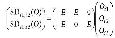
can be formed by a linear transformation
Where common satellites![]() are observed, E is an identity matrix that has the size of the observed satellite number; in the above example the size is 3 x 3. The covariance matrix of the single differences is then
are observed, E is an identity matrix that has the size of the observed satellite number; in the above example the size is 3 x 3. The covariance matrix of the single differences is then
i.e., the weight matrix is
That is, the single differences are un-correlated observables in the case of a single baseline. C in Eq. 6.97 is a general form, so C is denoted by![]() is the number of commonly viewed satellites.
is the number of commonly viewed satellites.
Single differences can be formed for any baselines as long as the two stations have common satellites in sight. However, the baselines should be a set of "independent" ones. The most-used methods are to form the radial baselines or traverse baselines. Supposing the stations’ id vector is![]() and the baseline between station i1 and i2 is denoted by
and the baseline between station i1 and i2 is denoted by![]() then the radial baselines could be formed, e.g., by
then the radial baselines could be formed, e.g., by![]()
![]() and the traverse baselines could be formed, e.g., by
and the traverse baselines could be formed, e.g., by![]()
![]() Station i1 is called a reference station and is freely selectable. In some cases, a mixed radial and traverse baselines have to be formed such as, e.g., by
Station i1 is called a reference station and is freely selectable. In some cases, a mixed radial and traverse baselines have to be formed such as, e.g., by![]()
![]() Sometimes the baselines have to be formed by several groups, and therefore several references have to be selected. A method of forming an independent and optimal baseline network will be discussed Sects. 9.1 and 9.2.
Sometimes the baselines have to be formed by several groups, and therefore several references have to be selected. A method of forming an independent and optimal baseline network will be discussed Sects. 9.1 and 9.2.
In case three stations are used to measure the GPS data, the original observable vector of station i1, i2 and i3 is
where n is the commonly observed satellite number. The single differences of the baseline (i, j) are
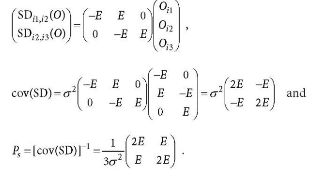
If the baselines are formed in a radial way, i.e., baselines are formed as![]() and
and ![]() then one has
then one has
If the baselines are formed in a traverse way, i.e., baselines are formed as![]() and
and![]() then one has
then one has
It is obvious that the single differences are correlated if the station numbers are more than two. And the correlation depends on the ways the baselines are formed. Therefore, a general covariance formula of the single differences of a network is not possible to be derived. Furthermore, the commonly viewed satellite number n could be different from baseline to baseline, so the formulation of the covariance matrix could be more complicated.
A baseline-wise processing of the GPS data of a network by using single differences is equivalent to an omission of the correlation between the baselines.
Double Differences
Double differences are formed between two single differences related to two observed satellites as
where k1 and k2 are the two id numbers of the satellites. Supposing the original observables have the same variance of![]() then the double differenced observables have a variance of
then the double differenced observables have a variance of![]() Considering Eqs. 6.89-6.92, one has
Considering Eqs. 6.89-6.92, one has
where![]() are the differenced ionospheric and tropospheric effects at the two stations related to the two satellites, respectively. For the ionosphere-free combined observables (denoted by j = 4 for distinguishing), the ionospheric error terms have vanished from above equations.
are the differenced ionospheric and tropospheric effects at the two stations related to the two satellites, respectively. For the ionosphere-free combined observables (denoted by j = 4 for distinguishing), the ionospheric error terms have vanished from above equations.
The most important property of the double differences is that the clock error terms in the equation (model) are completely eliminated. It should be emphasised that the clock error, which implicitly affects the computation of the position of the satellite, still has to be carefully considered. Ionospheric and tropospheric effects are reduced greatly through difference forming, especially for those stations that are not very far away from each other. Double differenced Doppler directly describes the geometry change. Double differenced ambiguities can be denoted by
The original ambiguities used in Eq. 6.103 are for convenience in case of reference satellite changing.
For the single difference observable vector
the double differences
can be formed by a linear transformation
where E is an identity matrix of size m x m, I is a 1 vector of size m (all elements of the vector are 1), m is the number of formed double differences, and m = n – 1. The cova-riance matrix of the double differences is then
For single and double differences
the linear transformation matrix![]() and the covariance matrix can be obtained by
and the covariance matrix can be obtained by
For the general case of
it is obvious that the general transformation matrix![]() and the related covariance matrix can be represented as
and the related covariance matrix can be represented as
where![]() is an m x m matrix whose elements are all 1, and the weight matrix has the form of
is an m x m matrix whose elements are all 1, and the weight matrix has the form of
where n = m +1. Equation 6.118 can be verified by an identity matrix test (i.e., P • cov(DD(0))= E).
In the case of three stations, supposing n common satellites![]() are viewed, then the single and double differences can be written as
are viewed, then the single and double differences can be written as
Then one has the transformation and covariance
Because of the dependency of the cov(SD) on the baselines forming, cov(DD) is also dependent on the baselines forming. A baseline-wise processing of a network GPS data using double differences is equivalent to an omission of the correlation between the baselines.
Triple Differences
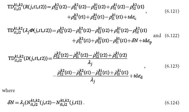
Triple differences are formed between two double differences related to the same stations and satellites at the two adjacent epochs as
where t1 and t2 are two adjacent epochs. Supposing the original observables have the same variance of![]() then the triple differenced observables have a variance of
then the triple differenced observables have a variance of![]() Considering Eqs. 6.102-6.104, one has
Considering Eqs. 6.102-6.104, one has
Ionospheric and tropospheric effects are eliminated. If there are no cycle slips during the time, the term of Eq. 6.124 is zero. Therefore, triple differences of Eq. 6.122 can also be used as a check for the cycle slips. Through triple difference forming, the systematic cycle slip turns out to be an effect like an outlier.
The most important property of the triple differences is that only the geometric changing is left in the models. Triple differences of Doppler describe the acceleration of the position.
For double differences
one has
where
Then the related covariance matrix can be represented as
where 1![]() is the double difference transformation matrix of two epochs. Because double differences are independent epoch wise,
is the double difference transformation matrix of two epochs. Because double differences are independent epoch wise,![]() is a diagonal matrix of
is a diagonal matrix of![]()
It is notable that the triple differences formed by epochs (t1, t2) are correlated to the differences formed by epochs (t0, t1) and (t1, t2). Such a correlation makes a sequential processing of the triple difference data very complicated. Sequentially using the above covariance formula indicates an omission of the correlation related to the previous epoch and the next epoch.
Taking the correlation between the baselines into account, an exact correlation description of the triple differences of a GPS network turns out to be very complicated.


