The principle of block-wise least squares adjustment can be summarised as below (Gotthardt 1978; Cui et al. 1982):
1. The linearised observation equation system can be represented by Eq. 7.1 (cf. Sect. 7.2).
2. The unknown vector X and observable vector L is rewritten as two sub-vectors:
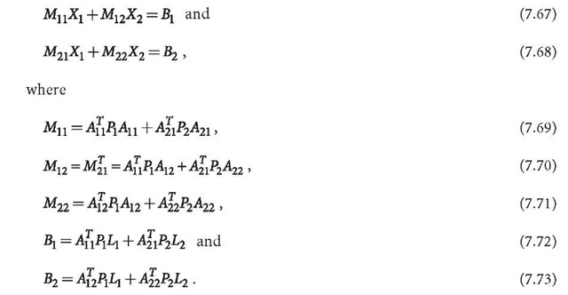
The least squares normal equation can then be formed as:
The normal equation can be denoted by
3. Normal Eqs. 7.67 and 7.68 can be solved as follows: from Eq. 7.67, one has
Substituting X1 into Eq. 7.68, one gets a normal equation related to the second block of unknowns:
The solution of Eq. 7.75 is then:
From Eqs. 7.78 and 7.74, the block-wise least squares solution of Eqs. 7.1 and 7.64 can be computed. For estimating the precision of the solved vector, one has (see discussion in Sect. 7.2):
Q is the inversion of the total normal matrix M. m is the number of total observations, and n is the number of unknowns.
Furthermore,
where (Gotthardt 1978; Cui et al. 1982)
One finds very important applications in GPS data processing by separating the unknowns into two groups, which will be discussed in the next sub-section.
Sequential Solution of Block-Wise Least Squares Adjustment
Suppose one has two sequential observation equation systems
with weight matrices![]() The unknown vector Y can be separated into two sub- vectors, one is sequential dependent, and another is time independent. Let us assume
The unknown vector Y can be separated into two sub- vectors, one is sequential dependent, and another is time independent. Let us assume
where![]() is the common unknown vector, and
is the common unknown vector, and![]() are sequential (time) independent unknowns (i.e., they are different from each other).
are sequential (time) independent unknowns (i.e., they are different from each other).
Equations 7.87 and 7.88 can be solved separately by using the block-wise least squares method as follows (cf. Sect. 7.5):
and
where indices t1 and t2 outside of the parenthesis indicate that the matrices and vectors are related to Eqs. 7.87 and 7.88, respectively.
The combined solution of Eqs. 7.87 and 7.88 then can be derived as:
where index ta means that the solution is related to all equations. The normal equations related to the common unknowns are accumulated and solved for. The solved common unknowns are used for computing sequentially different unknowns.
In the case of many sequential observations, a combined solution could be difficult or even impossible because of the large number of unknowns and the requirement of the computing capacities. Therefore, a sequential solution could be a good alternative. For the sequential observation equations
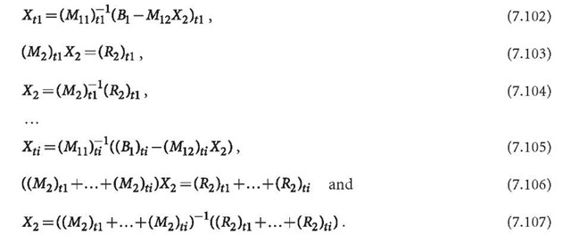
the sequential solutions are
It is notable that the sequential solution of the second unknown sub-vector X2 is exactly the same as the combined solution at the last step. The only difference between the combined solution and the sequential solution is that the X2 used are different. In the sequential solution, only the up-to-date X2 is used. Therefore at end of the sequential solution (Eq. 7.107), the last obtained X2 has to be sub-stituted into all Xj computing formulas, where j < i. This can be done in two ways. The first way is to remember all formulas for computing Xj, after X2 is obtained from Eq. 7.107, using X2 to compute Xj. The second way is to go back to the beginning after the X2 is obtained, and use X2 as the known vector to solve Xj once again. In these ways, the combined sequential observation equations can be solved exactly in a sequential way.
Block-Wise Least Squares for Code-Phase Combination
Recalling the block-wise observation equations discussed in Sect. 7.5, one has
Such an observation equation can be used for solving the problem of codephase combination. Supposing![]() are phase and code observation vectors, respectively, and they have the same dimensions, then
are phase and code observation vectors, respectively, and they have the same dimensions, then![]() is a sub-vector that only exists in phase observational equations. Then one has .
is a sub-vector that only exists in phase observational equations. Then one has .![]() as well as
as well as ![]() is the weight matrix, and
is the weight matrix, and![]() " are weight factors of phase and code observables. In order to keep the coefficient matrices
" are weight factors of phase and code observables. In order to keep the coefficient matrices![]() the observable vectors
the observable vectors![]() have to be carefully scaled. Equation 7.108 can be rewritten as:
have to be carefully scaled. Equation 7.108 can be rewritten as:
The least squares normal equation can be formed then as:
The normal equation can be denoted by
Normal equation 7.111 can be solved using the general formulas derived in Sect. 7.2 and Sect. 7.5.


