This section presents various fundamental concepts related to probability and random variables that will be required to support subsequent discussions. The discussion will focus on continuous random variables.
Basic Properties
Let w represent a real, scalar random variable. In the following, the notation![]() denotes the probability that the random variable w is less than the real number W.
denotes the probability that the random variable w is less than the real number W.
The distribution function of the random variable w is defined as the function
The function![]() is monotonically increasing in W, is continuous from the right with
is monotonically increasing in W, is continuous from the right with![]() The derivative of the distribution function is the (density function of the random variable w and will be denoted by
The derivative of the distribution function is the (density function of the random variable w and will be denoted by
The density function has the interpretation that![]() represents the probability that the random variable w assumes a value in the differential range
represents the probability that the random variable w assumes a value in the differential range ![]() Because the density is the derivative of a monotone function,
Because the density is the derivative of a monotone function, ![]() for any W. Based on the above definitions, for a scalar random variable,
for any W. Based on the above definitions, for a scalar random variable,
Let![]() be a function of the random variable w. The expected value of
be a function of the random variable w. The expected value of ![]() is defined by
is defined by
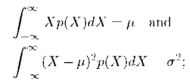
In particular, the expected value or mean of w is
As a simplified notation, this topic will typically use the notation![]() to indicate the expected value of the random variable
to indicate the expected value of the random variable![]() In cases where the meaning is clear or where double subscripting would otherwise occur, the subscript indicating the random variable may be dropped.
In cases where the meaning is clear or where double subscripting would otherwise occur, the subscript indicating the random variable may be dropped.
The variance of a scalar valued random variable![]() is defined by
is defined by
The variance of a random variable quantifies the variation of the random variable relative to its expected value. If we define![]() is called the standard deviation of
is called the standard deviation of![]()
The fc-th moment of![]() is defined by
is defined by
The first moment is the mean value. The variance and second moment are related by eqn. (4.13):
Example 4.3 Compute the mean, second moment, variance, and standard deviation of the random variable x with the exponential density
where
The mean is
The second moment is
The variance is![]() but can also be easily calculate from the information above using the eqn. (4-13) as
but can also be easily calculate from the information above using the eqn. (4-13) as
Therefore, the standard deviation is
Gaussian Distributions
The notation![]() is used to indicate that the scalar (or univariate) random variable x has the Gaussian or Normal density function described by
is used to indicate that the scalar (or univariate) random variable x has the Gaussian or Normal density function described by
therefore, the density of a Normal random variable is completely described by two parameters![]() It can be shown that
It can be shown that
therefore, the parameters![]() are the expected value and variance of the random variable x.
are the expected value and variance of the random variable x.
Transformations of Scalar Random Variables
This section presents the method to find the density for the random variable v under the conditions that![]() the function g is invertible, and the density for the random variable w is known.
the function g is invertible, and the density for the random variable w is known.
Due to the assumption that g is monotone, it has an inverse function ![]() The derivation begins with the basic idea that the probability of the events causing
The derivation begins with the basic idea that the probability of the events causing![]() and
and
![]() must be the same whether measured with respect to
must be the same whether measured with respect to![]() Mathematically this is expressed as
Mathematically this is expressed as![]()
![]()
![]()
where this formulation assumes that dW is positive. Therefore,![]() which will be used below. For positive, dW, the quantity dV can still be either positive or negative, depending on the sign of
which will be used below. For positive, dW, the quantity dV can still be either positive or negative, depending on the sign of![]() The computation of the probabilities in eqn. (4.15) must account for either possible sign:
The computation of the probabilities in eqn. (4.15) must account for either possible sign:
For the second integral, due to dV being negative, the original integral would have been over![]() which is equivalent to the integral in the expression above after interchanging the limits of integration and multiplying the integral by —1. The above integral relationships are equivalent to
which is equivalent to the integral in the expression above after interchanging the limits of integration and multiplying the integral by —1. The above integral relationships are equivalent to
which can be rewritten as
Issues related to the transformation of random variables are clarified by the following examples.
Example 4.4 Find the density for y where![]()
![]()
In this case,
Therefore,
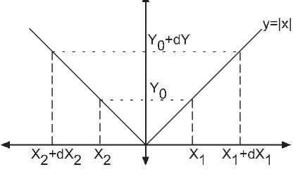
Figure 4.3: Graph of![]() with variables defined for Example 4.5.
with variables defined for Example 4.5.
Note that![]() has the form of a Gaussian distribution with mean b and variance
has the form of a Gaussian distribution with mean b and variance![]() therefore, y is a Gaussian random variable. In general, all linear operations on Gaussian random variables result in Gaussian random variables.
therefore, y is a Gaussian random variable. In general, all linear operations on Gaussian random variables result in Gaussian random variables.
Example 4.5 Find the density for y where![]()
Because the function g is not invertible, the result of eqn. (4.16) cannot be used. Instead, we have to revert to the main idea of eqn. (4.15) which is that the change of variable must preserve the probability of events. Consider the variables defined in Figure 4.3. For this problem, we have
where dY represents a positive differential change from![]() and
and
The above expression translates into the following integral
Using the changes of variables this integral simplifies as follows![]()
This integral relationship must hold for all nonnegative![]() and arbitrarily small dY. In addition, for
and arbitrarily small dY. In addition, for![]() we have
we have![]() therefore,
therefore,
This density does not have the form of eqn. (4.14); therefore, y is not a Gaussian random variable. In general, nonlinear transformations of Gaussian random variables do not result in Gaussian random variables.


