Deterministic Systems
The quantitative analysis of navigation systems will require analytic system models. Models can take a variety of forms. For finite dimensional linear systems with zero initial conditions that evolve in continuous-time, for example, the ordinary differential equation, transfer function, and state space models are equivalent. The dynamics of the physical systems of interest in navigation applications typically evolve in continuous-time, while the equations of the navigation system itself are often most efficiently implemented in discrete-time. Therefore, both difference and differential equations are of interest. This topic present several essential concepts from linear and nonlinear systems theory.
Three equivalent model structures for continuous-time systems are discussed in this section. The models are equivalent in the sense that each contains the same basic information about the system. However, some forms of analysis are more convenient in one model format than in another. Models for physical systems derived from basic principles often result in ordinary differential equation or state space models. Frequency response analysis and frequency domain system identification techniques utilize the transfer function representation. Optimal state estimation techniques are most conveniently presented and implemented using the state space approach. A major objective of this section is to provide the means to translate efficiently and accurately between these three model representations.
Ordinary Differential Equations
Many systems that evolve dynamically as a function of a continuous-time variable can be modeled effectively by a set of n-th order ordinary differential equations (ODE). When the applicable equations are linear, each n-th order differential equation is represented as
where the notation![]() denotes the j-th time derivative of the term in parenthesis. In this general form, the coefficients of the differential equation are time-varying. In applications involving time-invariant systems, the coefficients are constants.
denotes the j-th time derivative of the term in parenthesis. In this general form, the coefficients of the differential equation are time-varying. In applications involving time-invariant systems, the coefficients are constants.
Eqn. (3.1) represents a single-input single-output dynamical system. The input signal is represented by u(t). The output signal is represented by y(t). Eqn. (3.1) is referred to as the input-output ordinary differential equation.
When the applicable equations are nonlinear, the n-th order differential equation is represented in general as
Taylor series analysis of eqn. (3.2) about a nominal trajectory can be used to provide a linear model described as in eqn. (3.1) for local analysis. See Section 3.3.
To solve an n-th order differential equation for![]() requires n pieces of information (e.g., initial conditions) which describe the state of the system at time
requires n pieces of information (e.g., initial conditions) which describe the state of the system at time![]() This concept of system state will be made concrete in Section 3.5.
This concept of system state will be made concrete in Section 3.5.
Example 3.1 Consider a one dimensional frictionless system corresponding to an object with a known external force applied at the center of gravity. The corresponding differential equation is
where m is the mass,![]() is the acceleration, and f (t) is the external applied force. If the object is also subject to linear friction and restoring forces, then this is the classic forced mass-spring-damper example, The resulting differential equation is
is the acceleration, and f (t) is the external applied force. If the object is also subject to linear friction and restoring forces, then this is the classic forced mass-spring-damper example, The resulting differential equation is
where b represents the linear coefficient of friction and k is the coefficient of the linear restoring force.
Example 3.2 The differential equation for a single channel of the INS horizontal position error due to gyro measurement error is
where p is position in meters,![]() is the i-th derivative of position, g is gravitational acceleration, Re is the Earth radius, and
is the i-th derivative of position, g is gravitational acceleration, Re is the Earth radius, and![]() represents gyro measurement error.
represents gyro measurement error.
Transfer Functions
If a system described by eqn. (3.1) has constant coefficients, then frequency domain or Laplace analysis can aid the analyst’s understanding of the system performance. If the initial conditions in eqn. (3.1) are assumed to be zero, then the transfer function representing the linear system is found as follows:
where![]() denotes the Laplace transform of
denotes the Laplace transform of![]() and s denotes the Laplace variable. The transfer function for a linear time-invariant (LTI) system is the Laplace transform of the output divided by the Laplace transform of the input. When there is no pure delay in the LTI system, the transfer function can be represented as the ratio of two polynomials in s with constant coefficients. Note that the coefficients of the transfer function polynomials are identical to the input-output differential equation coefficients. The order of the transfer function is n. The system has n poles which are the roots of the denominator polynomial
and s denotes the Laplace variable. The transfer function for a linear time-invariant (LTI) system is the Laplace transform of the output divided by the Laplace transform of the input. When there is no pure delay in the LTI system, the transfer function can be represented as the ratio of two polynomials in s with constant coefficients. Note that the coefficients of the transfer function polynomials are identical to the input-output differential equation coefficients. The order of the transfer function is n. The system has n poles which are the roots of the denominator polynomial
The transfer function (finite) zeros are the roots of the numerator polynomial
Example 3.3 For the system described by eqn. (3.3), the transfer function from the forcing function to the position is
For the system described by eqn. (3.4), the transfer function from the forcing function to the position is
A transfer function is always defined in reference to a stated input and output. The transfer functions between different inputs and outputs are distinct, but (before pole zero cancellations) the denominators are always the same for all transfer functions related to a given system. For the system described by eqn. (3.4), the transfer function from the forcing function to the velocity is
Example 3.4 The transfer function corresponding to eqn. (3.5) is
The response of the systems depends on the form of the gyro error eg. The system includes a pure integrator, represented by the![]() factor in the transfer function, and an undamped oscillator with frequency
factor in the transfer function, and an undamped oscillator with frequency
This particular value of the natural frequency is referred to as the Schuler frequency. The transfer function from gyro error to velocity error is
Note that a constant gyro error would result in an oscillatory velocity error at the Schuler frequency. A
State Space
The state space representation converts each n-th order differential equation into n coupled first order differential equations. Such a representation is often desirable for ease of implementation and analysis, as the state space representation allows the use of vector and matrix techniques. State space techniques relevant to both continuous and discrete-time systems are discussed in Section 3.2-3.5.
Figure 3.1: Decomposition of a transfer function in eqns. (3.12-3.13).
For analysis only, let the transfer function of eqn. (3.6) be decomposed into two separate filtering operations:
as depicted in Figure 3.1 where![]()
![]() For the n-th order differential equation corresponding to eqn. (3.12), define a state vector x such that
For the n-th order differential equation corresponding to eqn. (3.12), define a state vector x such that![]() Then,
Then, 
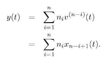
where the details are provided in Exercise 3.1. Taking the inverse Laplace transform of eqn. (3.13) and using the state vector definition, the system output is represented as
In matrix notation, the system can be described as
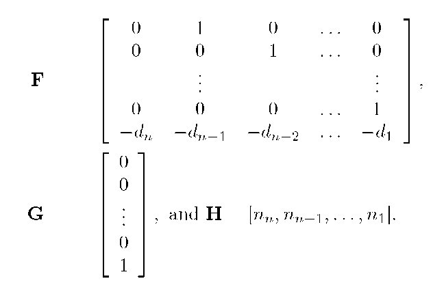
where
In such state space representations, F is referred to as the system matrix, G is referred to as the input matrix, and H is referred to as the output matrix. This particular state space implementation is referred to as the controllable canonical form. For any system, there exist an infinite number of equivalent state space representations. The transformation between equivalent state space representations is discussed in Section 3.5.1.
Example 3.5 A state space representation corresponding to the system describe by eqn. (3.3) is
where in this and the subsequent equations of this example
A state space representation corresponding to the system describe by eqn. (3.4) is
If in addition to position being an output, velocity was also an output, only the output matrix would change to
Example 3.6 Corresponding to the transfer function in eqn. (3.10) of Example 3.4, the controllable canonical form state space representation is
with state vector![]() Note that this state space representation is slightly different from the control canonical form. It has been modified, by shifting the gain g from the output to the input matrix, to cause each element of the state vector to have a clear physical meaning. Exercise 3.2 confirms that the input-output relationship is correct.
Note that this state space representation is slightly different from the control canonical form. It has been modified, by shifting the gain g from the output to the input matrix, to cause each element of the state vector to have a clear physical meaning. Exercise 3.2 confirms that the input-output relationship is correct.


