Face Tracking and Recognition in Video (Face Recognition Techniques) Part 3

Face Tracking from Multi-view Videos

The tracker is set in a Sequential Importance Resampling (SIR) (particle filtering) framework, which can be broken down into a description of its state space, the state transition model and the observation model. To fully describe the position and pose of a 3D object, we usually need a 6-D representation (R3 x SO(3)), where the 3-D real vector space is used to represent the object’s location, and the special orthogonal group SO(3) is used to represent the object’s rotation. In our work, we model the human head as a sphere and perform pose-robust recognition. This enables us to explore in 3-D state space S = R3. Each state vector s = [x,y,z] represents the 3-D position of a sphere’s center, disregarding the orientation. The radius of the sphere is assumed to be known through an initialization step. The low dimensionality of the state space contributes to the reliability of the tracker, since for SIR, even a large number of particles will necessarily be sparse in high dimensional space.

The state transition modelis    set as a Gaussian distribution

We have found that the tracking result is relatively insensitive to the specific value of σ and fixed it at 50 mm (our external camera calibration is metric). The observations for the filter are histograms extracted from the multi-view video frames Ij, where j is the camera index and t is the frame index. Histogram features are invariant to rotations and thus fit the circumstance of reduced state space. To adopt this feature, we need to back-project Ij onto the spherical head model and establish the histogram over the texture map. The observation likelihood is modeled as follows:

whereis the i th particle at the tth frame;.is the histogram of the texture map built from the particleis    the histogram of template texture map.

The template texture map is computed after initializing the head position in the first frame, then updated by back-projecting the head region in the image, which is fixed by the maximum a posteriori (MAP) estimate onto the sphere model. The D(H1H2) function calculates the Bhattacharyya distance between two normalized histograms.

We now describe the procedure for obtaining texture map on the surface of the head model. First, we uniformly sample the spherical surface. Then for the j th camera, the world coordinates of sample pointsare transformed into coordinates in that camera’s reference frameto    determine their visibility in that camera’s view. Only unoccluded points (i.e., those satisfyingis    the distance from the head center to the j th camera center) are projected onto the image plane. By relating these model surface points to the pixels at their projected image coordinateswe  build the texture map Mj of the visible hemisphere for the j th camera view. This continues until we have transformed the texture maps obtained from all camera views to the spherical model. Points in the overlapped region are fused using a weighting strategy, based on representing the texture map of the j th camera view as a function of locations of surface pointsWe  assign the function value at pointa    weightaccording to the point’s proximity to the projection center. This is based on the fact that, on the rim of a sphere, a large number of surface points tend to project to the same pixel, so image pixels corresponding to those points are not suitable for back-projection. The intensity value at the point of the resulting texture map will be:

where

 

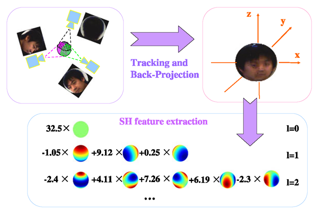
Fig. 13.3 Feature extraction. We first obtain the texture map of the human head on the surface of a spherical model through back projection of multi-view images captured by the camera network, then represent it with spherical harmonics

The texture mapping and back-projection processes are illustrated in the left part of Fig. 13.3.

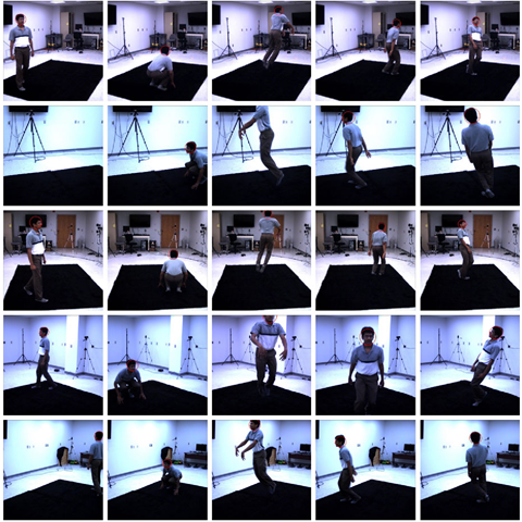
Figure 13.4 shows an example of our pose-free tracking result for a multi-view video sequence. The video sequence has 500 frames. The tracker is able to stably track all the frames without failure, despite the considerably abrupt motions and the frequent occurrences of rotation, translation and scaling of the human head as shown. Sometimes the subject’s head is outside the field-of-view of certain cameras. Though subjects usually do not undergo such extreme motion in real-world surveillance videos, this example clearly illustrates the reliability of our tracking algorithm. In our experiments, the tracker handles all the captured videos without difficulty. The occasionally observed inaccuracies in bounding circles are mostly due to the difference between sphere and the exact shapes of human heads. Successful tracking enables the subsequent recognition task.

Pose-Free Feature Based on Spherical Harmonics

In this section, we describe the procedure for extracting a rotation-invariant feature from the texture map obtained in Sect. 13.5.1. The process is illustrated in Fig. 13.3. According to the Spherical Harmonics (SH) theory, SHs form a set of orthonormal basis functions over the unit sphere, and can be used to linearly expand any square-integrable function on S2. SH representation has been used for matching 3D shapes [16] due to its properties related to the rotation group. In the vision community, following the work of Basri and Jacobs [5], researchers have used SH to understand the impact of illumination variations in face recognition [30, 39].

Fig. 13.4 Sample tracking results for a multi-view video sequence. 5 views are shown here. Each row of images is captured by the same camera. Each column of images corresponds to the same time-instant

The general SH representation is used to analyze complex functions (For description of general SH, please refer to [5] or [30]). However, the spherical function determined by the texture map are real functions, and thus we consider real spherical harmonics (or Tesseral SH):

wheredenotes    the    general    SH basis function of degreeand order m in

Note that here we are using the spherical coordinate system.are    the zenith angle and azimuth angle, respectively.

The Real SHs are also orthonormal and they share most of the major properties of the general Spherical Harmonics. From now on, the word “Spherical Harmonics” shall refer only to the Real SHs. As in Fourier expansion, the SH expansion coefficientsof functioncan    be    computed    as:

The expansion coefficients have a very important property which is directly related to our ‘pose-free’ face recognition application:

Proposition If two functions defined onare related by a  rotationand    their SH expansion coefficients arerespectively, the following relationship exists:

and thesatisfy:

In other words, after rotation, the SH expansion coefficients at a certain degree l are actually linear combinations of those before the rotation, and coefficients at different degrees do not affect each other. This proposition is a direct result of the following lemma [7, 16]:

Lemma Denote El the subspace spanned byis an irreducible representation for the rotation group SO(3).

Thus, given a texture mapand its  corresponding SH coefficient

we can formulate the energy vector associated with where fl is the vector of allat degree l. Equation (13.33) guarantees that ef keeps unchanged when the texture map is rotated, and this enables pose-robust face recognition. We refer to ef as the SH Energy feature. Note that this is different from the energy feature defined in [16]. In practice, we further normalize the SH energy feature with regard to total energy. This is the same as assuming that all the texture maps have the same total energy, and somehow function as an illumination-normalized signature. Although this also means that skin color information is not used for recognition, it proves to work very well in experiments.

Fig. 13.5 Comparison of the reconstruction qualities of head/face texture map with different number of spherical harmonic coefficients. The images from left to right are: the original 3D head/face texture map, the texture map reconstructed from 40-degree, 30-degree and 20-degree SH coefficients, respectively [32]

The remaining issue concerns with obtaining a suitable band-limited approximation with SH for our application. In Fig. 13.5, we show a 3D head texture map and its reconstructed version with 20, 30 and 40 degree SH transform, respectively. The ratio of computation time for the 3 cases is roughly 1:5:21. (The exact time varies with configuration of the computer, for example, on a PC with Xeon 2.13 GHz CPU, it takes roughly 1.2 seconds to do a 20 degree SH transform for 18 050 points.) We have observed that the 30-degree transform achieves the best balance between approximation precision and computational cost.

Measure Ensemble Similarity

Given two multi-view video sequences with m and n frames (Every “frame” is actually a group of images, each captured by a camera in the network.), respectively, we generate 2 ensembles of feature vectors, respectively. They may contain different number of vectors. To achieve video-level recognition, we are interested in measuring the similarity between these two sets of vectors. Now, we calculate the ensemble similarity as the limiting Bhattacharyya distance in RKHS following [41]. In experiments, we measure the ensemble similarity between feature vectors of a probe video and those of all the gallery videos. The gallery video with the shortest distance to the probe is considered as the best match. For detailed derivations and explanation of limiting Bhattacharyya distance in the RKHS, please refer to [41].

Experiments

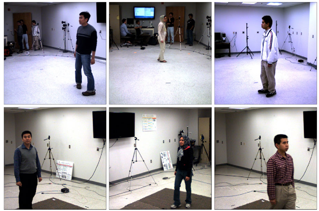
Most existing “multi-view” still or video face databases, such as PIE, Yale-B, the oriental face data, M2VTS etc., target recognition-across-pose algorithms, so they are not applicable to our multi-view to multi-view matching algorithm. The data we used in this work are multi-view video sequences captured with 4 or 5 video cameras in an indoor environment, collected at 3 different sessions: one for building a gallery and the other two for constructing probes. To test the robustness of our recognition algorithm, we arranged the second session to be one week after the first one, and the third 6 months after the second. The appearance of some subjects change significantly between the sessions. The database enrolls 25 subjects. Each subject has 1 gallery video and most subjects have 2 probe videos. Each video is 100 to 200 frames in length. Since each video sequence is captured with multiple cameras, it is equivalent to 4 or 5 videos in the single camera case. Figure 13.6 shows some example frames from gallery and probe video sequences. This data set poses great challenges to multi-view face recognition algorithms.

Fig. 13.6 Example of gallery and probe video frames. Images on the top are gallery frames, and those on the bottom are probe frames of the same subjects. Many subjects look differently in gallery and probe

Feature Comparison

We associate 5 different kinds of features with different classifiers to compare their performance in image-based face recognition systems. By “image-based face recognition” we mean that each frame is treated as gallery or probe individually and no video-level fusion of results is performed. As a result, the recognition rate is computed by counting the number of correctly classified frames, not videos. The inputs to all these face recognition systems are based on the same tracking results. For any system based on feature of raw image intensity value, we use only the head region that is cropped by a circular mask as provided by the tracking result. All the head images are scaled to 30 x 30. For the PCA features, Eigenvectors that preserve the top 95% energy are kept. For the SH-based feature, we perform a 30-degree SH transform. Here, we would like to emphasize that since both gallery and probe are captured when subjects are performing free motion, the poses exhibited in images of any view are arbitrary and keep changing. This is significantly different from the settings of most existing multi-view face databases. The results are shown in Table 13.4. As we can see, the performance of the proposed feature exceeds that of other features by a large margin in all cases. Note that we do not fuse the results of different views for non-SH-based features.

Table 13.4 Comparison of recognition performance

Feature	NN	KDE	SVM-Linear	SVM-RBF
Intensity PCA	49.7%	39.0%	49.2%	57.8%
Intensity LDA	50.5%	27.2%	33.1%	40.7%
SH PCA	33.6%	30.9%	31.2%	44.2%
SH Energy	55.3%	47.9%	50.3%	67.1%
Normalized SH Energy	60.8%	64.7%	78.2%	86.0%

Table 13.5 KL divergence of in-class and between-class distances for different features

Intensity	Intensity + PCA	SH + PCA	SH Energy	Normalized SH Energy
0.1454	0.1619	0.2843	0.1731	1.1408

To quantitatively verify the proposed feature’s discrimination power, we then conducted the following experiment. We calculate distances for each unordered pair of feature vectors {xi,xj} in the gallery. If {xi,xj} belongs to the same subject, then the distance is categorized as being in-class. Otherwise, the distance is categorized as being between-class. We approximate the distribution of the two kinds of distances as histograms.

Intuitively, if a feature has good discrimination power, then the in-class distances evaluated using that feature tends to take smaller values compared to the between-class distances. If the two distributions mix together, then this feature is not good for classification. We use the symmetric KL divergence KL(p||g) + KL(q\\p) to evaluate the difference between the two distributions. We summarize the values of KL divergence for the 5 features in Table 13.5 and plot the distributions in Fig. 13.7. As clearly shown, the in-class distances for normalized SH energy feature are concentrated in the low value bins, while the between-class ones tend to have higher values, and their modes are obviously separated from each other. For all other features, the between-class distances do not show a clear trend of being larger than the in-class ones, and their distributions are just mixed. The symmetric KL-divergence also suggests the same.

Fig. 13.7 Comparison of the discriminant power of the 5 features. First row, from left to right: intensity value, intensity value + PCA, SH. SH + PCA. Second row, from left to right: SH Energy. Normalized SH energy. The green cutye is between-class distance distribution and the red one is in-class distance distribution. Number of bins is 100 [32]

Video-Based Recognition

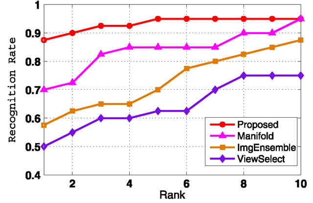
In this experiment, we compare the performance of 4 video-level recognition systems: (1) Ensemble-similarity-based algorithm as proposed in [41] for cropped face images. The head images in a video are automatically cropped by a circular mask as provided by the tracking results and scaled to 30 by 30. Then we calculate the limiting Bhattacharyya distance between gallery and probe videos in RKHS for recognition. The kernel is RBF. If a video has n frames and it is captured by k cameras, then there are k x n head (face) images in the ensemble. (2) View-selection-based algorithm. We first train a PCA subspace for frontal-view face. The training images are a subset of the Yale B database and are scaled to 30 by 30. We then use this subspace to pick frontal-view face images from our gallery videos. We construct a frontal-view face PCA subspace for each individual. For every frame of a probe video, we first compute the “frontalness” of the subject’s face in each view according to its distance to the general PCA model. The view which best matches the model is selected and fitted to the individual PCA subspaces of all the subjects. After classification of all the frames has been finished, recognition result for the video is obtained through majority voting. (3) video-based face recognition algorithm using probabilistic appearance manifold as proposed in [20]. We use 8 planes for local manifold model and set the probability of remaining the same pose to be 0.7 in the pose transition probability matrix. We first use this algorithm to process each view of a probe video. To fuse results of different views we use majority voting. If there is a tie in views’ voting, we pick the one with smaller Hausdorff distance as the winner. (4) Normalized SH energy feature + ensemble similarity. This algorithm is as described in Sect. 13.5.2 and Sect. 13.5.3.

We plot the cumulative recognition rate curve in Fig. 13.8. Note that the numbers shown here should not be compared with those in the previous image-based recognition experiment to draw misleading conclusions, as these two sets of recognition rates are not convertible to each other. The view-selection method heavily relies on the availability of frontal-view face images, however, in the camera network case, the frontal pose may not appear in any view of the cameras. As a result, it does not perform well in this multi-view to multi-view matching experiment. Rather than the ad-hoc majority voting fusion scheme adopted by the view-selection algorithm, the manifold-based algorithm and the image-ensemble-based algorithm use more reasonable strategies to combine classification results of individual frames. Moreover, they both have certain ability to handle pose variations, especially the manifold-based one. However, because they are designed to work with a single camera, they are single-view in nature. Repeating these algorithms for each view does not fully utilize the multi-view information. On the other hand, the proposed method is multiview in nature and is based on a pose-free feature, so it performs noticeably better than the other 3 algorithms in this experiment.

Fig. 13.8 Cumulative recognition rate of the 4 video-based face recognition algorithms

Conclusions

Video offers several advantages for face recognition, in terms of motion information and availability of more views. We reviewed several techniques that exploit video by either fusing information on a per-frame basis, considering them as image-ensembles, or by learning better appearance models. However, the availability of video opens interesting questions of how to exploit the temporal correlation for better tracking of faces, how to exploit behavioral cues available from video, and how to fuse the multiple views afforded by a camera network. Also, algorithms need to be derived that allow for matching a probe video to a still or video gallery. We showed applications involving such scenarios and discussed the issues involved in designing algorithms for such scenarios. There are several future research directions that are promising. While there are several studies that suggest that humans can recognize faces in non-cooperative conditions [26]—poor resolution, bad lighting etc.—if motion and dynamic information is available. This capability has been difficult to describe mathematically and replicate in an algorithm. If this phenomenon can be modeled mathematically, it could lead to more accurate surveillance and biometric systems. The role of familiarity in face recognition and the role that motion plays in recognition of familiar faces, while well known in psychology and neuroscience literature [31], is yet another avenue that has been challenging to model mathematically and replicate algorithmically.