Independent Component Analysis and Source Separation
While PCA minimizes the sample covariance (second-order dependence) of the data, independent component analysis (ICA) [6, 18] minimizes higher-order dependencies as well, and the components found by ICA are designed to be non-Gaussian. Like PCA, ICA yields a linear projection![]() but with different properties
but with different properties
that is, approximate reconstruction, nonorthogonality of the basis A, and the nearfactorization of the joint distribution P(y) into marginal distributions of the (non-Gaussian) ICs.
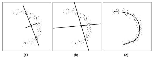
An example of ICA basis is shown in Fig. 2.5, where it is computed from a set of 3D points. The 2D subspace recovered by ICA appears to reflect the distribution of the data much better than the subspace obtained with PCA. Another example of an ICA basis is shown in Fig. 2.8b where we see two unordered nonorthogonal IC vectors, one of which is roughly aligned with the first principal component vector in Fig. 2.8a (see later), (i.e., the direction of maximum variance). Note that the actual non-Gaussianity and statistical independence achieved in this toy example are minimal at best, and so is the success of ICA in recovering the principal modes of the data.
Fig. 2.5 ICA vs. PCA decomposition of a 3D data set. a The bases of PCA (orthogonal) and ICA (nonorthogonal). b Left: the projection of the data onto the top two principal components (PCA). Right: the projection onto the top two independent components (ICA).
ICA is intimately related to the blind source separation problem: decomposition of the input signal (image) x into a linear combination (mixture) of independent source signals. Formally, the assumption is that xT = Ast, with A the unknown mixing matrix. ICA algorithms3 try to find A or the separating matrix W such that mt = WxT = WAst. When the data consist of M observations with N variables, the input to ICA is arranged in an N x M matrix X.
Bartlett et al. [1, 10] investigated the use of ICA framework for face recognition in two fundamentally different architectures:
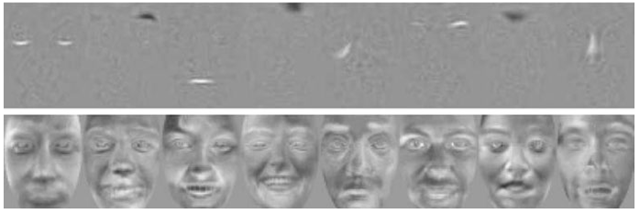
Architecture I Rows of S are independent basis images, which combined by A yield the input images X. Learning W allows us to estimate the basis images in the rows of U .In practice, for reasons of computational tractability, PCA is first performed on the input data X to find the top K eigenfaces; these are arranged in the columns of a matrix E .4 Then ICA is performed on Et ; that is, the images are variables, and the pixel values are observations. Let C be the PCA coefficient matrix, that is, X = CET. Then the k independent ICA basis images (Fig. 2.6, top) are estimated by the rows of U = WET, and the coefficients for the data are computed from X = EW—1U.
Architecture II This architecture assumes that the sources in S are independent coefficients, and the columns of the mixing matrix A are the basis images; that is, the variables in the source separation problem are the pixels. Similar to Architecture I, ICA is preceded by PCA; however, in this case the input to ICA is the coefficient matrix C. The resulting ICA basis consists of the columns of EA (Fig. 2.6, bottom), and the coefficients are found in the rows of U = WCt. These coefficients give the factorial representation of the data.
Fig. 2.6 Basis images obtained with ICA: Architecture I (top) and II (bottom).
Generally, the bases obtained with Architecture I reflect more local properties of the faces, whereas the bases in Architecture II have global properties and much more resemble faces (Fig. 2.6).
Multilinear SVD: “Tensorfaces”
The linear analysis methods discussed above have been shown to be suitable when pose, illumination, or expression are fixed across the face database. When any of these parameters is allowed to vary, the linear subspace representation does not capture this variation well (see Sect. 2.6.1). In Sect. 2.4, we discuss recognition with nonlinear subspaces. An alternative, multilinear approach, called “tensorfaces,” has been proposed by Vasilescu and Terzopoulos in [37, 38].
Tensor is a multidimensional generalization of a matrix: a n-order tensor![]() is an object with n indices, with elements denoted by
is an object with n indices, with elements denoted by![]() Note that there are n ways to flatten this tensor (i.e., to rearrange the elements in a matrix): The ith row of
Note that there are n ways to flatten this tensor (i.e., to rearrange the elements in a matrix): The ith row of![tmpdece-86_thumb[2] tmpdece-86_thumb[2]](http://what-when-how.com/wp-content/uploads/2012/06/tmpdece86_thumb2_thumb.png) is obtained by concatenating all the elements of
is obtained by concatenating all the elements of![]() of the form
of the form ![]()
A generalization of matrix multiplication for tensors is the l-mode product ![]() of a tensor
of a tensor![]() and an m x k matrix M, where k is the lth dimension of
and an m x k matrix M, where k is the lth dimension of![]()
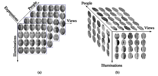
Fig. 2.7 Tensorfaces. a Data tensor; the four dimensions visualized are identity, illumination, pose, and the pixel vector. The fifth dimension corresponds to expression (only the subtensor for neutral expression is shown). b Tensorfaces decomposition.
Under this definition, Vasilescu and Terzopoulos proposed [38] an algorithm they called n-mode SVD, which decomposes an n-dimensional tensor A into
The role of the core tensor Z in this decomposition is similar to the role of the singular value matrix Σ in SVD (2.4): It governs the interactions between the mode matrices U1 ,…,Un, which contain the orthonormal bases for the spaces spanned by the corresponding dimensions of the data tensor. The mode matrices can be obtained by flattening the tensor across the corresponding dimension and performing PCA on the columns of the resulting matrix; then the core tensor is computed as
The notion of tensor can be applied to a face image ensemble in the following way [38]: Consider a set of N-pixel images of Np people’s faces, each photographed in Nv viewpoints, with Ni illuminations and Ne expressions. The entire set may be arranged in an Np x Nv x Ni x Ne x N tensor of order 5. Figure 2.7a illustrates this concept: Only four dimensions are shown; to visualize the fifth one (expression), imagine that the four-dimensional tensors for different expressions are “stacked.”
In this context, the face image tensor can be decomposed into
Each mode matrix represents a parameter of the object appearance. For example, the columns of the Ne x Ne matrix Ue span the space of expression parameters. The columns of Upixels span the image space; these are exactly the eigenfaces that would be obtained by direct PCA on the entire data set.
Each person in the database can be represented by a single Np vector, which contains coefficients with respect to the bases comprising the tensor
For a given viewpoint v, illumination i, and expression e, an Np x N matrix ![]() can be obtained by indexing into .
can be obtained by indexing into .![]() for v, i, e and flattening the resulting Np x 1 x 1 x 1 x N subtensor along the identity (people) mode. Now a training image xp,v,e,i of a person j under the given conditions can be written as
for v, i, e and flattening the resulting Np x 1 x 1 x 1 x N subtensor along the identity (people) mode. Now a training image xp,v,e,i of a person j under the given conditions can be written as
where Cj is the j th row vector of Up.
Given an input image x, a candidate coefficient vector cv,i,e is computed for all combinations of viewpoint, expression, and illumination, solving (2.18). Therecog-nition is carried out by finding the value of j that yields the minimum Euclidean distance between c and the vectors Cj across all illuminations, expressions, and viewpoints.5
Vasilescu and Terzopoulos [38] reported experiments involving the data tensor consisting of images of Np = 28 subjects photographed in Ni = 3 illumination conditions from Nv = 5 viewpoints, with Ne = 3 different expressions; the images were resized and cropped so they contain N = 7493 pixels. The performance of tensor-faces is reported to be significantly better than that of standard eigenfaces described in Sect. 2.3.1.
Nonlinear Subspaces
In this section, we describe a number of techniques that do not assume that the principal manifold is linear.
Principal Curves and Nonlinear PCA
The defining property of nonlinear principal manifolds is that the inverse image of the manifold in the original space RN is a nonlinear (curved) lower-dimensional surface that “passes through the middle of the data” while minimizing the sum total distance between the data points and their projections on that surface. Often referred to as principal curves [14], this formulation is essentially a nonlinear regression on the data. An example of a principal curve is shown in Fig. 2.8c.
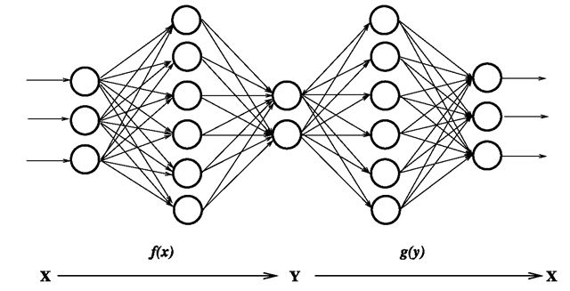
One of the simplest methods for computing nonlinear principal manifolds is the nonlinear PCA (NLPCA) autoencoder multilayer neural network [9, 20] shown in Fig. 2.9.
Fig. 2.8 a PCA basis (linear, ordered, and orthogonal). b ICA basis (linear, unordered, and nonorthogonal). c Principal curve (parameterized nonlinear manifold). The circle shows the data mean
Fig. 2.9 Autoassociative (“bottleneck”) neural network for computing principal manifolds![]() in the input space
in the input space![]()
The “bottleneck” layer forms a lower-dimensional manifold representation by means of a nonlinear projection function f(x ), implemented as a weighted sum-of-sigmoids. The resulting principal components y have an inverse mapping with a similar nonlinear reconstruction function g(y), which reproduces the input data as accurately as possible. The NLPCA computed by such a multilayer sigmoidal neural network is equivalent (with certain exceptions6) to a principal surface under the more general definition [13, 14]. To summarize, the main properties of NLPCA are
corresponding to nonlinear projection, approximate reconstruction, and typically no prior knowledge regarding the joint distribution of the components, respectively (however, see Zemel and Hinton [43] for an example of devising suitable priors in such cases). The principal curve in Fig. 2.8c was generated with a 2-4-1-4-2 layer neural network of the type shown in Fig. 2.9. Note how the principal curve yields a compact, relatively accurate representation of the data, in contrast to the linear models (PCA and ICA).
Kernel-PCA and Kernel-Fisher Methods
Recently nonlinear principal component analysis has been revived with the “kernel eigenvalue” method of Scholkopf et al. [32]. The basic methodology of KPCA is to apply a nonlinear mapping to the input![]() and then solve for a linear
and then solve for a linear
PCA in the resulting feature space Rl , where L is larger than N and possibly infinite. Because of this increase in dimensionality, the mapping Ψ(χ ) is made implicit (and economical) by the use of kernel functions satisfying Mercer’s theorem [7]
where kernel evaluations![]() in the input space correspond to dot-products in the higher dimensional feature space. Because computing covariance is based on dot-products, performing a PCA in the feature space can be formulated with kernels in the input space without the explicit (and possibly prohibitively expensive) direct computation of Ψ (x). Specifically, assuming that the projection of the data in feature space is zero-mean (“centered”), the covariance is given by
in the input space correspond to dot-products in the higher dimensional feature space. Because computing covariance is based on dot-products, performing a PCA in the feature space can be formulated with kernels in the input space without the explicit (and possibly prohibitively expensive) direct computation of Ψ (x). Specifically, assuming that the projection of the data in feature space is zero-mean (“centered”), the covariance is given by
with the resulting eigenvector equation![]() Since the eigenvectors (columns of V) must lie in the span of the training data Ψ(χ{ ), it must be true that for each training point
Since the eigenvectors (columns of V) must lie in the span of the training data Ψ(χ{ ), it must be true that for each training point
and that there must exist coefficients![]() such that
such that
Using the definition of Σκ, substituting the above equation into (2.22) and defining the resulting T -by- T matrix K by![]() leads to the equivalent
leads to the equivalent
eigenvalue problem formulated in terms of kernels in the input space
where![tmpdece-133_thumb[2] tmpdece-133_thumb[2]](http://what-when-how.com/wp-content/uploads/2012/06/tmpdece133_thumb2_thumb.png) is the vector of expansion coefficients of a given eigenvector V as defined in (2.23). The kernel matrix
is the vector of expansion coefficients of a given eigenvector V as defined in (2.23). The kernel matrix![]() is then diagonalized with a standard PCA.7 Orthonormality of the eigenvectors,
is then diagonalized with a standard PCA.7 Orthonormality of the eigenvectors,![]() leads to the equivalent normalization of their respective expansion coefficients,
leads to the equivalent normalization of their respective expansion coefficients,
Subsequently, the KPCA principal components of any input vector can be efficiently computed with simple kernel evaluations against the dataset. The nth principal component yn of x is given by
where V n is the nth eigenvector of the feature space defined by Ψ .As with PCA, the eigenvectors Vn can be ranked by decreasing order of their eigenvalues Xn and a d-dimensional manifold projection of x is![tmpdece-142_thumb[2] tmpdece-142_thumb[2]](http://what-when-how.com/wp-content/uploads/2012/06/tmpdece142_thumb2_thumb.png) with individual components defined by (2.25).
with individual components defined by (2.25).
A significant advantage of KPCA over neural network and principal curves is that KPCA does not require nonlinear optimization, is not subject to overfitting, and does not require prior knowledge of network architecture or the number of dimensions. Furthermore, unlike traditional PCA, one can use more eigenvector projections than the input dimensionality of the data (because KPCA is based on the matrix K, the number of eigenvectors or features available is T). On the other hand, the selection of the optimal kernel (and its associated parameters) remains an “engineering problem.” Typical kernels include Gaussians![tmpdece-143_thumb[2] tmpdece-143_thumb[2]](http://what-when-how.com/wp-content/uploads/2012/06/tmpdece143_thumb2_thumb.png) polynomials
polynomials
![tmpdece-144_thumb[2] tmpdece-144_thumb[2]](http://what-when-how.com/wp-content/uploads/2012/06/tmpdece144_thumb2_thumb.png) and sigmoids
and sigmoids![]() all of which satisfy Mercer’s theorem [7].
all of which satisfy Mercer’s theorem [7].
Similar to the derivation of KPCA, one may extend the Fisherfaces method (see Sect. 2.3.3) by applying the FLD in the feature space. Yang [42] derived the kernel Fisherfaces algorithm, which maximizes the between-scatter to within-scatter ratio in the feature space through the use of the kernel matrix K. In experiments on two data sets that contained images from 40 and 11 subjects, respectively, with varying pose, scale, and illumination, this algorithm showed performance clearly superior to that of ICA, PCA, and KPCA and somewhat better than that of the standard Fisherfaces.


![tmpdece-100_thumb[2] tmpdece-100_thumb[2]](http://what-when-how.com/wp-content/uploads/2012/06/tmpdece100_thumb2_thumb.png)

![tmpdece-102_thumb[2] tmpdece-102_thumb[2]](http://what-when-how.com/wp-content/uploads/2012/06/tmpdece102_thumb2_thumb.png)
![tmpdece-103_thumb[2] tmpdece-103_thumb[2]](http://what-when-how.com/wp-content/uploads/2012/06/tmpdece103_thumb2_thumb.png)
![tmpdece-105_thumb[2] tmpdece-105_thumb[2]](http://what-when-how.com/wp-content/uploads/2012/06/tmpdece105_thumb2_thumb.png)
![tmpdece-110_thumb[2] tmpdece-110_thumb[2]](http://what-when-how.com/wp-content/uploads/2012/06/tmpdece110_thumb2_thumb.png)


![tmpdece-120_thumb[2] tmpdece-120_thumb[2]](http://what-when-how.com/wp-content/uploads/2012/06/tmpdece120_thumb2_thumb.png)
![tmpdece-123_thumb[2] tmpdece-123_thumb[2]](http://what-when-how.com/wp-content/uploads/2012/06/tmpdece123_thumb2_thumb.png)
![tmpdece-129_thumb[2] tmpdece-129_thumb[2]](http://what-when-how.com/wp-content/uploads/2012/06/tmpdece129_thumb2_thumb.png)
![tmpdece-141_thumb[2] tmpdece-141_thumb[2]](http://what-when-how.com/wp-content/uploads/2012/06/tmpdece141_thumb2_thumb.png)
