Introduction
In building models of facial appearance, we adopt a statistical approach that learns the ways in which the shape and texture of the face vary across a range of images. We rely on obtaining a suitably large and representative training set of images of faces, each of which is annotated with a set of feature points that define correspondences across the set. The positions of the feature points also define the shape of the face, and are analysed to learn the ways in which the shape can vary. The patterns of intensities are analysed in a similar way to learn how the texture can vary. The result is a model which is capable of synthesising any of the training images and generalising from them, but is specific enough that only face-like images are generated.
To build a statistical appearance model, we require a set of training images that covers the types of variation we want the model to represent. For instance, if we are only interested in faces with neutral expressions, we need only include neutral expressions in the model. If, however, we want to synthesise and recognise a range of expressions, the training set should include images of people smiling, frowning, winking and so on. Ideally, the faces in the training set should be of at least as high a resolution as those in the images we wish to synthesise or interpret.
Statistical Models of Shape
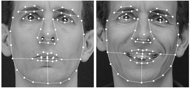
To define a shape model, we first annotate each face with a fixed number of points that define the key facial features (and their correspondences across the training set) and represent the shape of the face in the image. Typically, we place points around the main facial features (eyes, nose, mouth and eye-brows) together with points that define the boundary of the face (Fig. 5.1).
Fig. 5.1 Examples of 68 points defining facial features on two frontal images
The more points we use, the more subtle the variations in shape that we can represent.
If we annotate the face with n feature points, then we can represent the geometry of the face with a 2n element vector,
such that N training images provide N training vectors x,. The shape of the face can then be defined as that property of the configuration of points which is invariant under (that is, not explained by) some global transformation. In other words, if St (x) applies a transformation defined by parameters t to the points x, the configurations of points defined by x and St(x) are considered to have the same shape. Typically, we use either the similarity transformation or the affine transformation where a 2D similarity has four parameters (x – and y-translation, rotation and scaling) and a 2D affine transformations has six (x – and y-translation, rotation, scaling, aspect ratio and skew).
Given a set of shapes as training data, we can then apply formal statistical techniques [23] to analyse their variation and synthesise new shapes that are similar. Before we perform statistical analysis on these training vectors, however, it is important that we first remove any differences that are attributable to the global transformation, St (x), leaving only genuine differences in shape (that is, we must align the shapes into a common coordinate frame).
Aligning Sets of Shapes
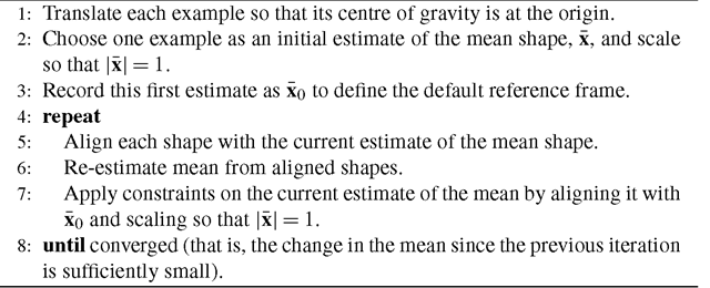
Of the various methods of aligning shapes into a common coordinate frame, the most popular is Procrustes Analysis [27] that finds the parameters, t, that transform each shape in the set, x,, so that it is aligned with a mean shape, x, in the sense that minimises their sum of squared distances, Though we can solve this analytically for a set of shapes, in practice we use a simple and effective iterative approach (Algorithm 5.1) to converge on a solution. At each iteration, we ensure that this measure is well defined by aligning the mean shape to the coordinate frame such that it is centred at the origin, has unit scale and some fixed but arbitrary orientation.
Algorithm 5.1: Aligning a set of shapes
Linear Models of Shape Variation
We now have N training vectors, x;, each with n points in d dimensions (usually d = 2 or d = 3) that are aligned to a common coordinate frame. By treating these vectors as points in nd-dimensional space and modelling their distribution, we can generate new examples that are similar to those in the original training set (that is, sample from the distribution) and examine new shapes to decide whether they are plausible examples (that is, evaluate a sample’s probability).
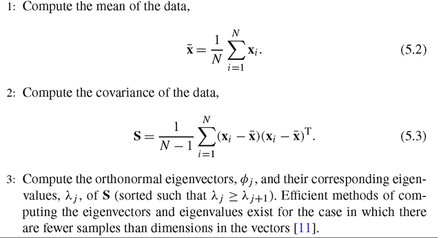
Not every nd-dimensional vector forms a face, however, and the set of valid face shapes typically lies on a manifold that can be described by k < nd underlying model parameters, b. By computing a parameterised model of the form x = M(b), we can approximate the distribution over shape, p(x), with the distribution over model parameters, p(b), and therefore generate new shapes by sampling from p(b) and applying the model, or evaluate a shape’s probability by evaluating the probability of its corresponding parameters, p(M-1(x)). The simplest approximation we can make to the manifold is a linear subspace that passes through the mean shape (equivalent to assuming a Gaussian distribution over both x and b). An effective approach to estimating the subspace parameters is to apply Principal Component Analysis (PCA) to the training vectors, x; (Algorithm 5.2). This computes the directions of greatest variance in nd-dimensional space, of which we keep only the k most ‘significant’. Each training example can then be described by its k < nd projections onto these directions, reducing the effective dimensionality of the data.
We can then approximate any example shape from the training set, x using
where contains the eigenvectors corresponding to the k largest eigenvalues and b is a k-dimensional vector given by
Algorithm 5.2: Principal component analysis
Fig. 5.2 Two modes of a face shape model (varied by ±2 s.d. from the mean). The first shape mode corresponds mostly to 3D head rotation whereas the second captures facial expression
where because the eigenvectors are orthonormal. The vector bs therefore defines a set of parameters of a deformable shape model and by varying the elements of bs we can vary the generated shape, x, via (5.4).
Given a shape in the model frame, x = M(b), we can then generate the corresponding shape in the image frame, X, by applying a suitable transformation such that X = St (x). Typically St will be a similarity transformation described by a scaling, s, an in-plane rotation, θ, and a translation, (tx,ty). By representing the scaling and rotation jointly as![]() I and sy = s sin θ, we ensure
I and sy = s sin θ, we ensure
that the pose parameter vector,![]() is zero for the identity transformation and that St (x) is linear in the pose parameters.
is zero for the identity transformation and that St (x) is linear in the pose parameters.
Due to the ordering of the eigenvalues, λj, the corresponding modes of shape variation are sorted in descending order of ‘importance’. For example, a model built from examples of a single individual with different viewpoints and expressions will often select 3D rotation of the head (that causes a large change in the projected shape) as the most significant mode, followed by expression (Fig. 5.2).
Choosing the Number of Shape Modes
The number of modes, k, that we keep determines how much meaningful shape variation (and how much meaningless noise) is represented by the model, and should therefore be chosen with care. A simple approach is to choose the smallest k that explains a given proportion (e.g., 98%) of the total variance exhibited in the training set,![]() where each eigenvalue λj gives the variance of the data about the mean in the direction of the j th eigenvector. More specifically, it is normal to choose the smallest k that satisfies
where each eigenvalue λj gives the variance of the data about the mean in the direction of the j th eigenvector. More specifically, it is normal to choose the smallest k that satisfies
where fv defines the proportion of Vt that we want to explain (e.g., fv = 0.98). Alternatively, we could build a sequence of models with increasing k and choose the smallest model that approximates all training examples to within a given accuracy (e.g., at most one pixel of error for any feature point). Performing this test in a miss-one-out manner—testing each example against models built from all other examples—gives us further confidence in the chosen k.
Fitting the Model to New Points
Suppose now we wish to find the best pose and shape parameters to align a model instance x to a new set of image points, X’. Minimising the sum of square distances between corresponding model and image points is equivalent to minimising the expression
or, more generally,
where Wpts is a diagonal matrix that applies a different weight for each point. If the allowed global transformation St(·) is more complex than a simple translation then this is a non-linear equation with no analytic solution. A good approximation can be found rapidly, however, by using a two-stage iterative approach (Algorithm 5.3) where each step solves a linear equation for common choices of transformation (e.g., similarity or affine) [30].
If the weights in Wpts relate to the uncertainty in the estimates of positions of target points, X’, then £pts can be related to the log likelihood. Adding a term representing the prior distribution on the shape parameters, p(bj, then gives the log posterior,
Algorithm 5.3: Shape model fitting
If the training shapes, Ixi}, have a multivariate Gaussian distributedthen the parameters, b, will have an axis-aligned Gaussian distribution, where
where such that
This prior, however, biases shape parameters toward zero which may be unjustified. Therefore, a common approach is to apply a uniform elliptical prior over shape parameters such that
where a suitable limit can be estimated from the data. In this case, maximising the posterior amounts to a linear projection (giving the maximum likelihood solution), followed by truncation of the corresponding shape parameters to lie within the elliptical bounds.
Further Reading
Our experiments on 2D images suggest that a Gaussian distribution over shape parameters (implying a linear subspace of face shapes) is a good approximation as long as the training set contains only modest viewpoint variation. Nonlinear changes in shape such as introduced by large viewpoint variation [15], result in a linear subspace model that captures all of the required variation but in doing so also permits invalid shapes that lie off the nonlinear manifold [43].
To account explicitly for 3D head rotation (or viewpoint change), several studies have computed a 3D linear shape model and fitted it to new image data under perspective [5, 61] or orthogonal [43] projection. These approaches separate all rigid movement of the head from nonrigid shape deformation while maintaining some linearity for efficient computation (see Chap. 6 for more details on explicit 3D models).
Other studies avoid modelling nonlinearities explicitly, instead opting to use methods that estimate the parameters of the nonlinear manifold directly. Early examples outside of the face domain include polynomial regression [54] and mixture models [8] whereas later studies applied nonlinear PCA [24], Kernel PCA [46], the Gaussian Process Latent Variable Model [32] and tensor-based models [36] to the face alignment problem.


