In this topic we move on to a different but related set of algorithms, broadly classified as image filtering. The topic of filtering digital waveforms in one dimension or images in two dimensions has a long and storied history. The basic idea in digital image filtering is to post-process an image using standard techniques culled from signal processing theory. An analogy may be drawn to the type of filters one might employ in traditional photography. An optical filter placed on a camera’s lens is used to accentuate or attenuate certain global characteristics of the image seen on film. For example, photographers may use a red filter to separate plants from a background of mist or haze, and most professional photographers use a polarizing filter for glare removal1. Optical filters work their magic in the analog domain (and hence can be thought of as analog filters), whereas in this topic we implement digital filters to process digital images.
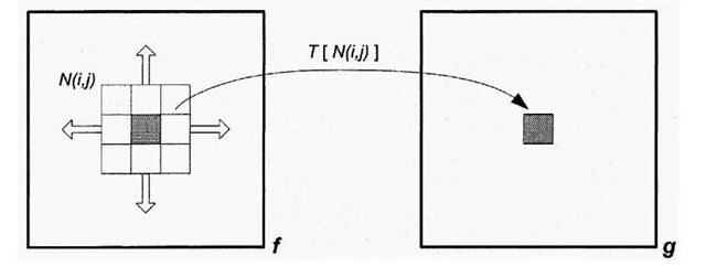
A common means of filtering images is through the use of "sliding neighborhood processing", where a "mask" is slid across the input image and at each point, an output pixel is computed using some formula that combines the pixels within the current neighborhood. This type of processing is shown diagrammatically in Figure 4-1, which is a high-level illustration of a 3×3 mask being applied to an image.
Figure 4-1. Image Enhancement via "sliding window", or neighborhood processing. As the neighborhood currently centered about the shaded pixel ffij) is overlaid around the image f, the pixel intensities combine to produce filtered pixels g(i,j).
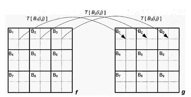
Figure 4-2. "Block processing" of images. Processed image g is created by partitioning/into distinct sections, an operation T is applied to all the pixels in each block/(Bk), and the corresponding block g (Bk) receives this output. The Discrete Cosine Transform (DCT), the transform that forms the heart of the JPEG image compression system, is performed in this manner using 8×8 blocks.
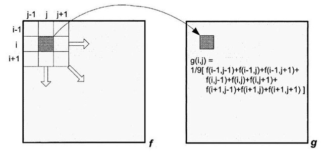
The sliding window operation - where N(ij) is larger than just a single pixel – is used to perform spatial filtering of images. The mask, also referred to as a filter kernel, consists of weighting factors that depending on its makeup, either accentuates or attenuates certain qualities of the processed image. Basically what happens is that each input pixel f(i,j) is replaced by a function of f(i,j)’s neighboring pixels. For example, an image can be smoothed by setting each output pixel in the filtered image g(i,j) with the weighted average of the corresponding neighborhood centered about the input pixel f(i,j). If the neighborhood is of size 3×3 pixels, and each pixel in the neighborhood is given equal weight, then Figure 4-3 shows the formula used to collapse each neighborhood to an output pixel intensity.
Figure 4-3. Sliding window in action. As the mask is shifted about the image for each position (ij), the intensity g(ij) is set to the average of/(y/s nine surrounding neighbors.
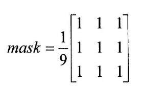
The filter kernel shown in Figure 4-3 is typically represented in matrix form, i.e.
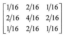
Each element in the matrix kernel is a filter coefficient, sometimes referred to as a filter "tap" in signal processing parlance. The neighborhood pixels need not be weighted evenly to smooth the image. For example, it may make sense to give a larger weight to pixels in the center of the neighborhood, and use smaller weights for those pixels located on the neighborhood’s periphery, as in the following mask:
It is important to note that this kernel is both symmetric and more importantly, the sum of its weights is 1. If the sum of an averaging kernel’s weights is not exactly 1, then the processed image will not have the same gain (overall brightness) as the input image and this is usually not desired. The application of these masks can be computationally expensive. If the input gray-scale image is of size MxN pixels, and the mask is a square kernel of size PxP (all of the kernels we use in this topic are square), then spatially filtering the image requires MNP2 multiplication/addition operations. Using reasonable values for M, N, and P (640×480 image dimensions, and a 5×5 mask) yields over 7.5 million operations to filter an image! The good news is that DSP cores are specifically architected so that a core element in digital filtering, the multiply and accumulate (MAC) operation, almost always can be performed in a single clock cycle – a statement not necessarily true when speaking of general-purpose CPUs (see 1.6).
Image Noise
Spatial filters are very often used to suppress noise (corrupted pixels) in images – this is known as the "image restoration" or "image denoising" problem, and figures quite prominently in the image processing field. Image noise may be the result of a variety of sources, including:
• Noisy transmission channels, for example in space imaging where the noise density overcomes any forward error detection capabilities.
• Measurement errors, such as those emanating from flawed optics or artifacts due to motion jitter. In the former case, a classic example in astronomical imaging was the initial Hubble telescope, where imperfections in the main mirror caused sub-standard image acquisition. In the latter case, early satellite imagery provides plenty of case studies, as the motion of the spacecraft and/or vibration of the acquisition machinery introduced distortions in the acquired images.
• Quantization (the act of sampling an analog signal and converting it to a digital form) effects manifest themselves as high-frequency noise.
• Camera readout errors cause impulsive noise, sometimes referred to as "shot" or "salt and pepper" noise.
• Electrical noise arising from interference between various components in an imaging system.
• The deterioration of aging films, such as the original 1937 "Snow White and the Seven Dwarfs," many of which have been digitally restored in recent years.
Restoring a degraded image entails modeling the noise, and utilizing an appropriate filter based on this model. Image noise comes in many flavors, and as a consequence the appropriate model should be employed for robust image restoration. Noise may be additive, which can be expressed as
where/is the original 2D signal (image), n is the noise contribution, and g is the corrupted image. Image noise can also be multiplicative, where
Noise may be highly correlated with the signal / or completely uncorrected. If the noise is highly structured, it may be due to defects in the manufacturing process of the detector, such as when faulty pixels produce images with pixel dropouts. Here, one possible model is to replace any offending pixels with the average of its neighbors. However, since the exact location of any faulty pixel is presumably known a priori, it follows that a far more efficient and effective means of reducing this highly structured noise is to generate a list of image locations that should be filtered, and apply an averaging mask over just those locations. Yet another form of structured noise is the "dark current" associated with Charged Coupled Device (CCD) cameras. This type of noise is very dependent on temperature and exposure time, however if these two variables are fixed it is possible to remove this type of noise via image subtraction. The activation energy of a CCD pixel is the amount of energy needed to excite the constituent electrons to produce a given pixel intensity. Pixels with low activation energies need comparatively less energy to produce equivalent pixel counts and are said to run "hot." Removing this form of noise is best accomplished through judicious calibration – capturing a so-called "dark field" image, one acquired without any illumination, at nominal temperature and exposure times and subsequently subtracting this calibration image from each new acquisition.
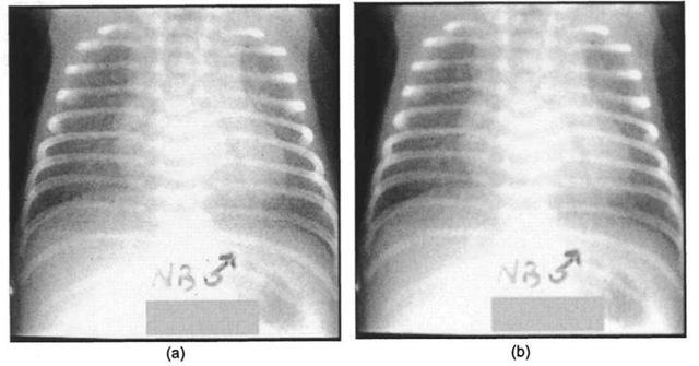
Spatial filtering is best used when dealing with unstructured or stochastic noise, where the location and magnitude of the noise is not known in advance, but development of a general model of the degrading process is feasible. Averaging filters are sometimes utilized in x-ray imaging, which suffer from a grainy appearance due to a well-known effect that goes by the moniker "quantum mottle." Reducing the amount of radiation a patient is exposed to during an x-ray acquisition is always beneficial for the patient -the problem is that with fewer photons hitting the image acquisition device, the statistical fluctuation of the x-ray begins to take on added effect, resulting in a non-uniform image due to the increased presence of additive film-grain noise. The problem gets progressively worse when image intensifiers are used, as boosting the image unfortunately also boosts the effects of the noise. By "smoothing" the radiograph using a procedure that will be discussed in great detail in 4.1.2, one can often enhance the resultant image, as demonstrated in Figure 4-4.
The image smoothing operation does succeed in reducing noise, but concomitant with the filtering is a loss of spatial resolution which in turn leads to an overall loss of information. Through careful selection of the size of the averaging kernel and the filter coefficients, a balance is struck between reduction of quantum mottle and retention of significant features of the image. In later sections of this topic we explore other types of filters that are sometimes better suited for the removal of this type of noise.
Other types of stochastic noise are quite common. Digitization devices, such as CCD cameras, always suffer from readout noise as a result of the uncertainty during the analog-to-digital conversion of the CCD array signal. Any image acquisition system using significant amounts of electronics is susceptible to electronic noise, especially wideband thermal noise emanating from amplifiers that manifests itself as Gaussian white noise with a flat power spectral density. The situation is exacerbated when the system gain of the acquisition device is increased, as any noise present with the system is amplified alongside the actual signal.
It should be emphasized that noise present within a digital image most likely does not arise from a single source and could very well contain multiple types of noise. Each element in the imaging chain (optics, digitization, and electronics) contributes to potential degradation. An image may suffer from both impulsive shot noise and signal-dependent speckle noise, or an image may be contaminated with blurring due to motion during acquisition, as well as some electronic noise.
Figure 4-4. Reduction of quantum mottle noise by image smoothing (image courtesy of Neil Trent, Dept. of Radiology, Univ. of Missouri Health Care), (a) Original chest radiograph of infant. Note the speckled and grainy nature of the image, (b) Processed image, using an 1 lxl 1 Gaussian low-pass filter (ct=1). The grainy noise has been reduced, at the cost of spatial resolution.
In short, for image filtering to be effective, these factors must be taken into account – no filter exists that can robustly handle all types of noise.
Two-Dimensional Convolution, Low-Pass and High-Pass Filters
The smoothing operation, which is really nothing more than a moving average, is an example of two-dimensional linear filtering (non-linear filters are covered in 4.5). The filter kernel is multiplied by the neighborhood surrounding each pixel in the input image, the individual products summed, and the result placed in the output image, as depicted in Figure 4-3. This process may be described in mathematical form as
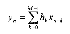
where/and g are MxN images, so that 0 < < M, 0 <j < N, and h is a square kernel of size NHxNH pixels. The above expression is the convolution equation in two dimensions. Convolution is of fundamental importance in signal processing theory, and because this topic is covered so well in many other sources2,3, a mathematically rigorous and thorough discussion is not given here. Suffice it to say that for the most part, the theory behind one-dimensional signal processing extends easily to two dimensions in the image processing field. In ID signal processing, a time domain signal x„ is filtered by convolving that signal with a set of Mcoefficients h:
These types of filters, and by extension their 2D analogue, are called finite impulse response (FIR) filters because if the input x is an impulse (x„=l for n=0 and xn=0 otherwise), the filter’s output eventually tapers off to zero. The output of a filter obtained by feeding it an impulse is called the filter’s impulse response, and the impulse response completely characterizes the filter. FIR filters are more stable than infinite impulse response (IIR) filters, where the impulse response never tapers off to zero. FIR filters are simply weighted averages, and the 2D convolution operator we use in image processing to spatially filter images is in fact a 2D FIR filter.
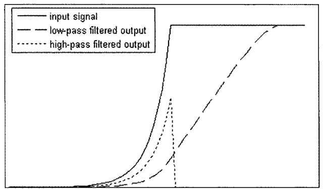
Figure 4-5. The effect of low-pass and high-pass filters in one dimension. In one dimension, the analogue to an image smoothing kernel is a filter that produces a running average of the original signal (the low-pass filtered output). A one-dimensional high-pass filter emphasizes the differences between consecutive samples.
The makeup of the filter coefficients, or filter taps, determines how the filter behaves. As we have already seen, various types of averaging kernels produce a blurred, or smoothed, image. This type of output is an example of using a low-pass filter, which diminishes high spatial frequency components, thereby reducing the visual effect of edges as the surrounding pixel intensities blur together. As one might expect, there are other types of linear filters, for example high-pass filters which have the opposite effect of low-pass filters. High-pass filters attenuate low-frequency components, so regions in an image of constant brightness are mapped to zero and the fine details of an image emphasized. Figure 4-5 illustrates the effects of low-pass and high-pass filters in a single dimension.
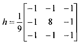
High-pass filters are considerably more difficult to derive than low-pass filters. While averaging filters always consist of purely positive kernels, that is not the case for high-pass kernels. A common 3×3 high-pass kernel is
In general, a high-pass kernel of size NHxNH may be generated by setting the center weight to (NH2-1)/NH2 and the rest to -1/NH2. Upon passing an image through a high-pass filter of this form, the average pixel intensity (DC level) is zero, implying that many pixels in the output will be negative. As a consequence a scaling equation, perhaps coupled with clipping to handle saturation, should then be used as a final post-processing step. In addition, since most noise contributes to the high frequency content of an image, high-pass filters have the unfortunate side effect of also accentuating noise along with the fine details of an image.
Better looking and more natural images can be obtained by using different forms of high-pass filters. One means of performing high-pass filtering is to first repeatedly low-pass filter an image, and then subtract the smoothed image from the original, thereby leaving only the high spatial frequency components. In simpler terms, high-pass filtered image = original image – smoothed imaged
The high-pass filtered image in the above relation contains only high-frequency components. However, it is usually desirable to retain some of the content of the original image, and this can be achieved through application of the following equation:
where h is a low-pass kernel, a-/? = 1, the * symbol denotes convolution, and n signifies the fact that we blur the image by convolving it with the low-pass kernel n times. This procedure is known as unsharp masking, and finds common use in the printing industry as well as in digital photography, astronomical imaging, and microscopy. By boosting the high-frequency components at the expense of the low-frequency components, instead of merely completely removing the low-frequency portions of the image, the filter has the more subtle effect of sharpening the image. Thus the unsharp mask can be used to enhance images that may appear "soft" or out-of-focus. The unsharp mask is demonstrated in Figure 4-6.
