Section 4.5.2 focused on using the median filter to enhance images corrupted by shot noise. It was shown that low-pass filters do not perform as well as median filters in removing impulse noise, because the spatial smoothing mixes any image-independent noisy outliers with the signal content. The median filter, on the other hand, was found to be well-suited for removing such signal-independent statistical outliers, while at the same time preserving the edges of the image. But what if the noise is not completely independent of the signal content, for example additive or multiplicative noise corrupting an image such that the noisy pixels are a mixture of original pixel intensities and noise levels? Might it be possible to construct an intelligent filter that somehow adapts itself to this behavior?
Adaptive filters are designed to address this question, and are the third and final class of spatial image filters we shall explore. The premise behind adaptive image filtering is that by varying the filtering method as the kernel slides across the image (in the same manner as the convolution operation), they are able to tailor themselves to the local properties and structures of an image. In essence, they can be thought of as self-adjusting digital filters. While certain types of adaptive filters may perform better than median filters at removing impulse noise (these are mostly variations on the basic median filtering scheme), they are most often used for denoising non-stationary images, which tend to exhibit abrupt intensity changes. Because the filtering operation is no longer purely uniform and instead modulated based on the local characteristics of the image, these filters can be employed effectively when there is little a priori knowledge of the signal being processed.
Adaptive filters find widespread use in countering the effects of so-called "speckle" noise, which afflicts coherent imaging systems like SAR and ultrasound. With these imaging techniques, scattered waves interfere with one another to contaminate an acquired image with multiplicative speckle noise. Various statistical models of speckle noise exist, with one of the more common being
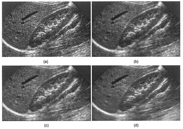
where g is the corrupted image and n(x,y) is drawn from a zero-mean Gaussian distribution with a given standard deviation. It is clear from the above model that speckle noise is dependent on the magnitude of the signal f, and in fact this type of noise is a serious impediment on the interpretability of image data because it degrades both spatial and contrast resolution. This situation is shown with a real-world example in Figure 4-24, where an ultrasound image exhibiting a fairly large amount of speckle noise is enhanced, illustrating the utility of adaptive filtering.
Figure 4-24. Ultrasound speckle noise removal, (a) Unprocessed ultrasound image of kidney anatomy, (b) Smoothed image (5×5 averaging filter), which while reducing speckle seriously degrades spatial resolution, (c) Result of adaptive filtering, using MATLAB wiener2 Image-Processing Toolkit function, (d) Commercial quality speckle tioise reduction, where image is despeckled using an adaptive geometric filter and then edge sharpened.
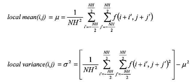
Adaptive filters are effective in reducing the deleterious effects of speckle noise because they are capable of adjusting themselves based on the signal content of the image. Thus it follows that they must use some measure of the local characteristics of the image in order to perform their job. Many adaptive filters are predicated on the use of local pixel statistics, primarily the mean and variance of the pixels within the current neighborhood. The local mean is simply the average pixel intensity of the neighborhood. The local variance is calculated in two stages from the pixels contained within the current neighborhood. First, the mean of the sum of the squares is computed, and then the square of the local mean is subtracted from this number yielding a statistical quantity known as the variance, very often referred to as a2. In mathematical terms, these image statistics can be expressed as
where /is the image and each neighborhood is of size NHxNH pixels. The standard deviation of the neighborhood is the square root of the variance, or a.
The Minimal Mean Square Error Filter
The adaptive filter we spend the majority of time on in this section is the Minimal Mean Square Error (MMSE) filter. This filter can be used to remove both additive white noise and speckle noise. Consider an observed image f(i,j) and a neighborhood L of size NHxNH. Let cr2 be the noise variance, be the local mean, and <j\ be the local variance. The cr2 parameter is the variance of a representative background area of the image containing nothing but noise (a technique for estimating this parameter is given later). The linear MMSE filter output is then given by26
This equation describes a linear interpolation between the observed image /and a smoothed version off. Care should be taken to handle the case where
in which case a negative output pixel may result (the MMSE filter implemented later in this section clamps the ratio![]() The MMSE filter works as follows:
The MMSE filter works as follows:
1. If the local variance is much greater than the noise variance, or if![]() is small or zero, it produces a value close to the input f(i,j). If
is small or zero, it produces a value close to the input f(i,j). If![]() this part of the image most likely contains an edge and this filter makes the assumption that it is best to leave that portion of the image alone.
this part of the image most likely contains an edge and this filter makes the assumption that it is best to leave that portion of the image alone.
2. If the noise variance dominates over the local variance, return the local mean.
3. If the two variance measures are more or less equal, the filter returns a mixture between the input and local mean.
This filter is edge-preserving because of (1), and consequently should tend to retain overall image sharpness, although noise will not be filtered from those portions of the image containing edges. Algorithm 4-2 describes the MMSE filter in pseudo-code form.
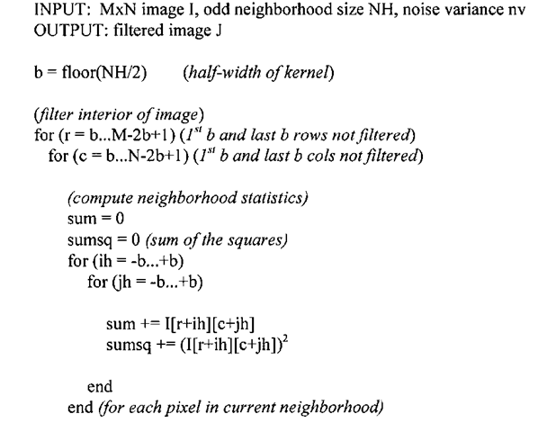
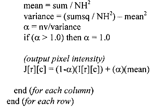
Algorithm 4-2: MMSE Adaptive Filter
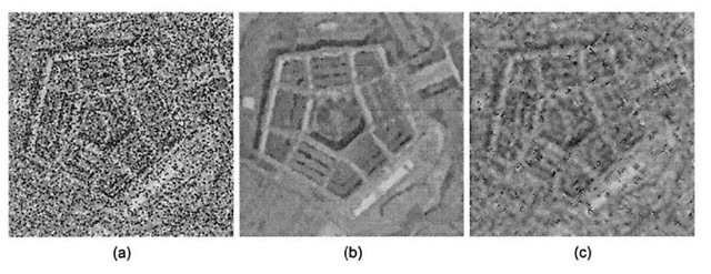
Figure 4-25 illustrates Algorithm 4-2 in action, comparing its performance with a median filter on an image corrupted with a fair amount of speckle noise. The MMSE filter does a slightly better job of attenuating multiplicative noise while retaining image sharpness, resulting in a performance increase of about 1/3 dB in PSNR. While the MMSE filter is well-suited for dealing with speckle noise, it is not a panacea. A key facet to image enhancement is that the right tool should be used for the job, as clearly illustrated in Figure 4-26. The MMSE filter fails miserably with shot noise and the median filter is the more appropriate filter to use in this case. If the image is contaminated with both shot and speckle noise, a different filter should be used that can handle both types of noise, some of which are discussed in the next section.
Figure 4-25 illustrates Algorithm 4-2 in action, comparing its performance with a median filter on an image corrupted with a fair amount of speckle noise. The MMSE filter does a slightly better job of attenuating multiplicative noise while retaining image sharpness, resulting in a performance increase of about 1/3 dB in PSNR. While the MMSE filter is well-suited for dealing with speckle noise, it is not a panacea. A key facet to image enhancement is that the right tool should be used for the job, as clearly illustrated in Figure 4-26. The MMSE filter fails miserably with shot noise and the median filter is the more appropriate filter to use in this case. If the image is contaminated with both shot and speckle noise, a different filter should be used that can handle both types of noise, some of which are discussed in the next section.
Other Adaptive Filters
There exists a large number of adaptive spatial filters, many of them variations on a similar theme and tuned for specific applications. In this section, we take a brief look at some of the more common adaptive image filters, before going to back to the MMSE filter and getting that algorithm to run on the DSP.
The Double Window-Modified Trimmed Mean (DW-MTM) filter performs well in the presence of both shot noise and signal-dependent noise like additive Gaussian and multiplicative speckle noise26. This filter’s namesake arises from the fact it utilizes two neighborhoods, a small one centered about the current pixel from which a median pixel intensity is calculated, and a larger one about the same center pixel from which a modified local mean is computed. This modified local mean is a modified average intensity in that any pixel whose gray-level differs by more than kunmL, where £ is a constant, cr„ is the standard deviation of the noise, and mL is the median of the small neighborhood, is excluded from the mean computation. The output intensity is then the average of the remaining pixels. In this way the DW-MTM filter operates as a quasi-smoothing filter but one where statistical outliers do not throw off the mean calculation. Of course, what exactly constitutes a statistical outlier can be difficult to predict. In this case, an outlier is parameterized by k and the magnitude of the noise (both of which remain constant throughout the filtering operation), as well as the median of the small neighborhood, which of course varies throughout the image and provides the adaptive aspect to this filter.
Figure 4-25. Speckle noise removal using a 3×3 MMSE adaptive filter, (a) Original Pentagon satellite image, (b) Image corrupted with multiplicative speckle noise (modeled using zero-mean Gaussian distribution with variance 0.025). (c) Processed image using 3×3 median filter, (d) Processed image using 3×3 MMSE filter.
Figure 4-26. MMSE adaptive filtering and shot noise, (a) Original Pentagon satellite image corrupted with 20% salt & pepper noise, (b) Result of 5×5 median filter, (c) Result of 5×5 MMSE filter.
This idea of trimming away outlier pixels finds its way into another adaptive filter, the alpha-trimmed mean filter. Given an m x n neighborhood, where N0 is the current neighborhood, an output image g is formed according to the relation
where the modified neighborhood /’ (x,y) is created from f(x,y) by excluding the maximum a/2 brightest and a/2 darkest pixels. This operation is best illustrated by example, as in Figure 4-27. The adaptive local noise reduction filter is similar in nature to the MMSE filter, in that it uses both the noise variance and local variance to form the output pixel. This filter is given by
where![]() is the local mean. With this filter, if
is the local mean. With this filter, if![]() is close to zero, it produces an output very close to the input f(i,j). Likewise, if
is close to zero, it produces an output very close to the input f(i,j). Likewise, if![]() it also produces an output pixel close to f(i,j). Otherwise, this filter outputs a pixel close to the local average.
it also produces an output pixel close to f(i,j). Otherwise, this filter outputs a pixel close to the local average.
The signal adaptive median or SAM filter26 is interesting in that it uses low-pass and high-pass filtered versions of the input image, in conjunction with an adaptive step involving the noise and local variances to yield a filter that exhibits excellent performance with respect to noise reduction while also preserving edges and overall image "crispness", however at a steep computational cost.
Figure 4-27. Alpha-trimmed mean filter, for the case of an example 3×3 neighborhood and a=2.
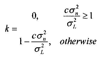
The factor k is once again based on the ratio![]() that we encountered in the adaptive local noise reduction and MMSE filters, and is given by
that we encountered in the adaptive local noise reduction and MMSE filters, and is given by
where c is a positive constant.

