Automatic Wood Log Segmentation Using Graph Cuts (Computer Vision,Imaging and Computer Graphics) Part 2

Results

We tested our approach on images taken by employees from forestry. Due to the image acquisition with a mobile phone, our tested input images are jpeg compressed with maximal resolution of 2048 x 1536 pixels. In our application we implemented the weight computation in four different ways as described before. All methods determine the edge weights wb as specified in 4.2 but differ in the calculation of the wr,

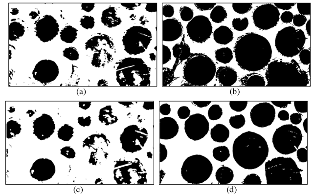
Fig. 5. The different steps of the presegmented center image are shown. Image (a) shows the thresholded modified Y-channel, (b) the thresholded V-channel and (c) the intersection of (a) and (b). In Image (d) the result of the first graph cut with KD-NN is shown.

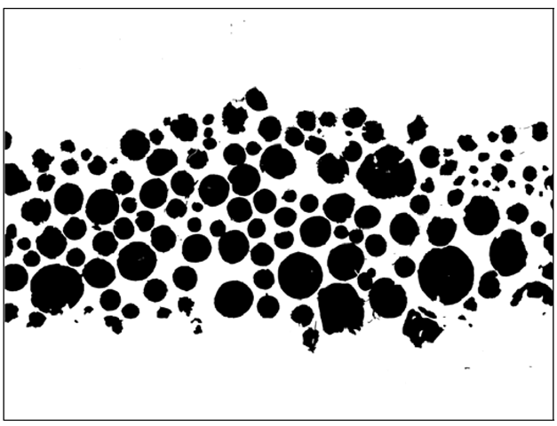
In our novel approach the graph-cut is processed twice. To compare the different methods the same weight setting for graph-cut in the presegmentation is used. Hence the same conditions, especially the same foreground Bfg and background pixels Bbg, are given for the second graph-cut. We generally used the best method for setting the weights i.e. our KD-NN for the graph cut segmentation as evaluated later. In figure 5 and 6 the different states of the presegmentation and the final result of the input image (figure 2) are shown. Thereby the image quality improves over the consecutive steps.

For the comparison of the different weight setting methods including our novel KD-NN from section 4.2, we performed a ground truth test. Therefore 71 very different sample images with wood logs were marked and the differences to the segmentation result were measured as shown in figure 9. We experimentally chose the best parameter to determine wr. The weights created with the histogram were calculated with β = 1000. For K-Mean γ was set to 0.02 and for our KD-NN wm = 0.5 and r = 2.5 were used. By all methods we used α = 0.0005 for wb. Furthermore the simple RGB color space, where R,G,B e [0, 255], was used in all methods, which also provided the best results.

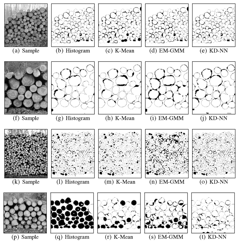
For the differentiation of the results we calculated correctly (true) and incorrectly (false) analyzed pixels for each foreground (positive) and background (negative). Therefore the values given in table 1 show the percentage of correctly analyzed foreground (true positive), correctly analyzed background (true negative), incorrectly analyzed foreground (false positive) and incorrectly analyzed background (false negative) pixels in respect to the total number of pixels. For an impression on the correctness of our analyzes the difference images in figure 9 show correctly analyzed pixels in white and incorrectly analyzed pixels in black. The objective would be to have a white difference image.

Fig. 6. The final segmentation of the second graph-cut run with KD-NN by using the presegmented center image, which is shown in figure 5

Fig. 7. The evaluation stages used in figure 9; (a) input image, (b) ground truth image with marked foreground, (c) image with analysis results, (d) difference image ground truth vs. analyzed image

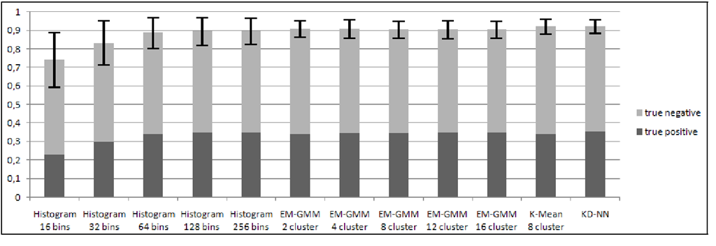
Fig. 8. Evaluation results for all weight setting algorithms showing correctly analyzed pixels (true positive and true negative) in respect to the total number of pixels. KD-NN gives best results having the lowest standard deviation.

Fig. 9. Four wood log sample images (a),(f),(k),(p) and the corresponding difference images of the different weight setting approaches. Thereby the best parameter were experimentally chosen for each method. For the segmentation with the histogram 32 bins per color channel were used. For the K-Mean and EM-GMM segmentation eight foreground and background clusters were applied.

As can be seen from table 1 and figure 8, KD-NN leads to the least general segmentation error (false negative + false positive). The K-Mean with eight clusters, whereby each cluster is initially positioned in one corner of the color cube, leads to similar results. The Histogram generally performs worst and the EM-GMM is a little bit better. Altogether K-Mean and KD-NN are the best methods from the four we tested for setting the weights in our application, whereby KD-NN is slightly better than K-Mean.

Conclusions and Future Work

We presented a novel method to accurately segment log cut surfaces in pictures taken from a stack of wood by smart phone cameras using the min-cut/ maxflow framework.

Table 1. The measured difference to the ground truth for all methods are shown here. The standard deviation are presented in brackets.

If certain restrictions on the image acquisition are made, the described approach is robust under different lighting conditions and cut surface colors. Robustness stems from our new, relatively simple and easy to implement density estimation. We compared our method with other approaches and showed that we mostly outperformed them. Our method leads to similar results as K-Mean clustering of the color space. However, our method is faster because of the kd-tree we are using. It is also more robust against outliers, which can be a problem using K-Means clustering. We used a constant search radius which works very well for our application. This radius might be need to be set slightly variable in a more general setting. However, in future work we will synchronous analyze X-Mean [15].