A Deformable Model for Bringing Particles in Focus (Computer Vision,Imaging and Computer Graphics) Part 2

Experiments

In this section we will experimentally show the performance of our particle model. We want to investigate the precision and accuracy of our model. By precision we mean how good our model is in predicting the true size, shape and particle depth. The accuracy refers to variation in the model predictions. The experiments are conducted in relation to size estimation, shape estimation and the particles distance to the focus plane. For these experiments we chose the parameter shown in Table 1. Furthermore, we investigate the robustness of the method in relation to the initial position and size estimates of the particles.

Table 1. Model parameters

Parameter	Value	Parameter	Value
Radial lines (n)	8	Sampling steps (m )	30
Sampling distance (pixels)	30	Length constant (c)	0.35
Gaussian blur – simulated (σ)	2	Gaussian blur – real (σ)	I
Radial similarty (η – Eq. 2)	I	Variance weight (ξ – Eq. 2)	4000
Gaussian weight (s – Eq. 3)	0.5 m	Variance weight ( κ – Eq. 6 )	100

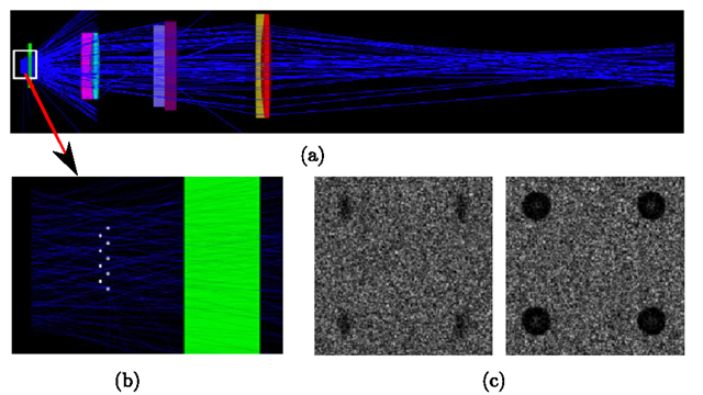
Fig. 6. Optical simulation in Zemax. (a) back illumination with a diffuse light source of 2 mm2 with wavelengths of 480-650 nm with transparent particles. (b) zoom on the particles and (c) examples of 50 μ\Ά out-of-focus ellipsoid particels (50 μ\Ά x 16.7 μ\Ά) and spherical in focus particles (50 μ\Ά).

Data. The endoscopic probe consists of three doublets with different powers separated as shown in Fig. 6. The distance between the object plane (particles) and the first optical element, which is a cover plate, is just 1 mm. The separations between the optical elements up to the CCD is maintained and optimized to provide a magnification of 6. The design is performed in Zemax optical design software. The total track length from object to image (particles to CCD) is 25 cm and the optical resolution of the system is 2 microns. The entire visible wavelength region is used to optimize this system (480-650 nm). The depth of focus at the object side is computed to be +/- 75 microns when defined by a drop of more than 90% of the modulation transfer function. Modeling is done in a non-sequential mode in Zemax, which allows us to incorporate the real situation of illumination with back light of spherical and ellipsoidal particles. Using the nonsequential mode we are able to handle diffuse light and 3D particles. The diffuse light source is located a few millimeters behind the particles and emits light in the specified wavelength range randomly over a 15 degrees angle. The particles used are transparent with refractive index of 1.6 at 555 nm wavelength. Several million rays per simulation were used to generate a single image with particles. Imaging is done using a CCD array with 4 Megapixels of 7 micron pitch.

The real data set consists of particles in water suspension placed between two glass sheets, which have been moved with μm precision relative to the focus plane. 25 μm particles are shown in Fig. 7.

Fig. 7. Setup for acquiring real data. Particles are placed between glass sheets as illustrated in (a), which can be moved relative to the camera with μ\Ά precision. In (b) an image example is shown with LED back illumination and 25 μ\Ά spherical transparent particles.

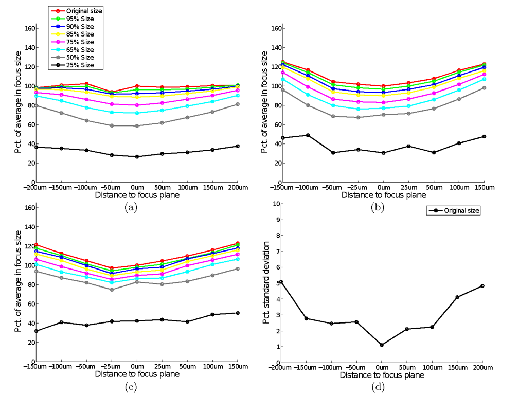
Fig. 8. Experiment with change of size. The horizontal axis of (a)-(c) shows the average radial distance relative to the in focus particle of original size. Standard deviation of the size estimate in percent of the original (d). Note the bias towards overestimation of size and less certainty as a function of out-of-focus.

Size Experiment. In this experiment we investigate the robustness of our size estimation. We have both tested the mean value and standard deviation of the estimated size, and how it depends on the distance to the focus plane. The results are shown in Fig. 8. The first three graphs (a)-(c) shows a relative size estimate as a function of distance to the focus plane, and each curve shows an individual size. There is a general bias towards overestimating the size of particles that are out-of-focus and small particles are also somewhat overestimated. The model is not capable of handling very large size changes, and gives an erroneous prediction for particle scaled to 25% size. This is due to the fixed parameter setting where the sampling is too coarse to identify the small particles. Size variation is obtained by scaling the images.

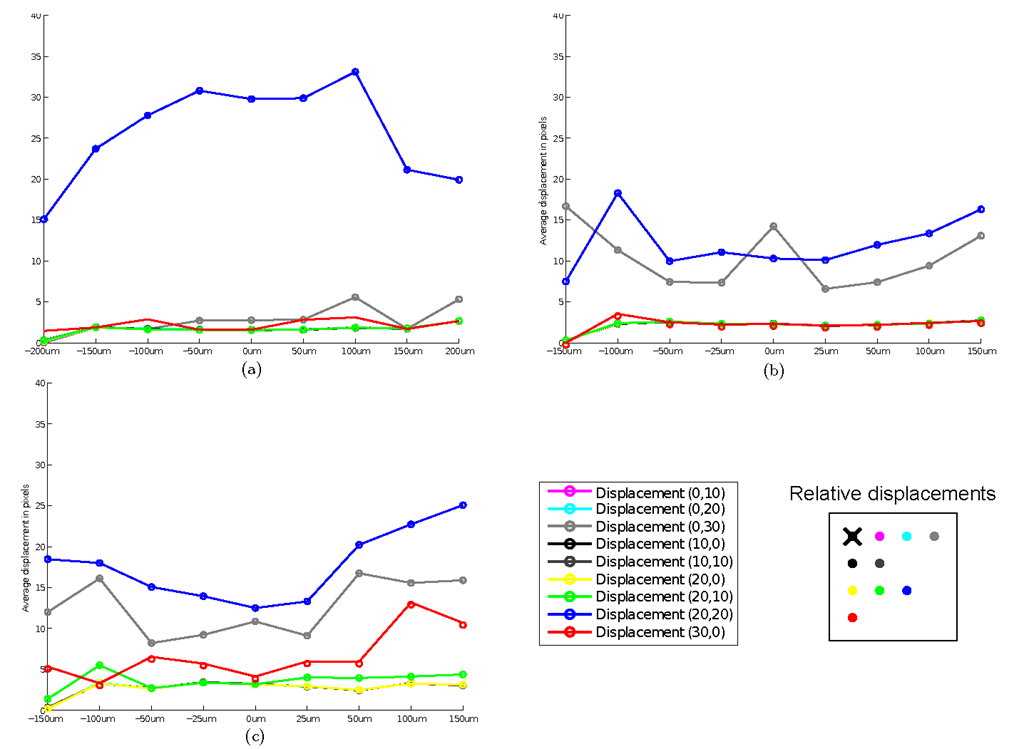
Fig. 9. Experiment for testing robustness to wrong spatial initialization of particle. The vertical axis is the average distance in pixels to the true position and the horizontal axis is the particle distance to the focus plane. A 50 μ\Ά particle has a radius of about 17 pixels. Experiments have been carried out for simulated particles, which are spherical (a), ellipsoids (1 x 2) (b), and ellipsoids (1 x 3) (c). Ellipsoids have the major axis vertical. The displacements are schematically shown in (b). Each displacement step is 10 pixels.

Fig. 9 illustrates the robustness to inaccurate spatial initialization. The model will only fail in finding a good center approximation if it is initialized far from the particle and especially if it is done diagonally.

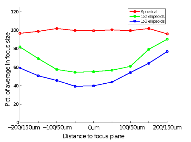
Shape Experiment. The purpose of this experiment is to investigate how the model deforms to adapt to non-spherical particles. We have conducted experiments on synthetic data with known ground truth and on real spray data. The spray data reflects some challenges encountered in particle analysis. The results of the synthetic data are shown in Fig. 10, where the relation between the horizontal and vertical line segments are plotted as a function of particle distance to the focus plane. The particles do not adapt completely to the expected shape, and there is a tendency for out-of-focus particles to be more circular than in focus particles. Despite the particle shape is not found exactly from the experiment, this can be inferred by regression, which we will show next. Examples of model alignment with real data is shown in Fig. 11.

Fig. 10. Shape experiment. The horizontal axis is the relation between the vertical and the horizontal line segments from our particle model, corresponding to the minor and major axis in the simulated ellipsoids. The true relation for the red curve would be 100%, the green curve would be 50% and the blue curve would be 33%.

Fig. 11. Examples of model alignment with images of water sprays. The model aligns well to most water droplets including the ones that are out of focus. In (a) two examples from the new model formulation is shown, and results of the second example is shown in (b) based on the original model formulation [3]. It is clear that the new particle alignment procedure improves the result. The main problem is now particles initially detected as two blobs by the blob detector, so some of them has two or more models aligned to them.

Regression Experiment. Results from our regression experiment is shown in Table 2. The regression is performed using ridge regression with Λ = 10~5. We divided our data set into approximately half training and half test sets, which was 12 particles from the simulated set for training and 13 particles for test, from each image. In the real data set, we have 82 depicted particles, and the split was 41 in each group. We had 27 simulated images, giving 675 observations for the simulation set. In the observed data set we have 82 particles in 9 images giving 738 observations. The results are obtained from 100 random splits in test and training data. We use the mean radial descriptor (Io) and the length for each line segment (ro) as input to our regression, see Eq. 7.

In the simulated data we perform a regression for both distance to the focus plane, particle size, and shape, which is the ratio between the major and minor axis. The obtained results show precise predictions, indicating that this characterization is adequate for reliable particle modeling. For the real data we also obtained satisfactory prediction of the distance to the focus plane, but with about 50% lower precision, compared to the artificial data.

Table 2. Regression model. Regression has been done for both simulated and real data. There were 25 particles in the simulated data and 82 particles in the real data set. The reported numbers are the standard deviation of the absolute errors of the regression, and the size range of the numbers. The columns are distance to the focus plane (Distance FP), average radial line length (Size), relation between the radial and horizontal line lengths (Shape).

Simulated data
	Distance FP Size Shape
Std.	14.20/itm 0.8921/itm 0.0357
Range	0-200/itm 33.3-50/itm 0.33-1.0
Real data
	Distance FP
Std.	21.69/itm
Range	0-180/itm

Discussion

We have described a deformable model, based on radial intensity sampling, and shown how it can be used for inferring size, shape and distance to the focus plane for back illuminated particles. This information is useful for process inspection, where not only size and shape information is obtained, but also 3D distribution information.

The data for our experiment is based on LED illumination, both what is used in the real data, and what is simulated. This is a rather cheap solution, and if it can provide satisfactory results, it will be a cost effective solution. But the rather diffuse illumination from the LEDs could be replaced by collinear laser, which will give much higher particle contrast, and therefore potentially improved performance. Whether this will give larger depth of field or just improved predictions is for future investigations to show.

The size experiment illustrates how robust our particle model is to the initialization. With the same set of parameters, it is capable of handling up to 50% scale change. In the spray experiment we used scale space blob detection for initializing the particle model, and adaptiveness to scale change and spatial initialization worked fine for the precision of blob detection. The only problematic issue is when an elongated particle is detected as two or more blobs. If elongated particles are important in the analysis, then alternative detectors should be considered.

Scaling images for size variation does not account for the change in optical properties of smaller particles. We know that smaller particles in back-illumination change appearance caused by scattering effects like refraction and defraction, and this requires further investigations to verify that our model will be able to characterize these particles. The appearance change will result in blurred particles, which our particle model handles fine. The main focus should therefore be on whether the regression model can predict the true size. Our regression experiment indicates that this should be possible.

The shape experiment shows that the model does not adapt precisely to the shape of the particle. This is caused by the Gaussian noise removal, which also blurs the particles making them appear less ellipsoid than they are in reality. The reason for using Gaussian convolution, which actually acts contrary to the deconvolution that we are trying to infer, is the noise level in the simulations. The noise is much larger, than what is seen in the real data, which can be seen by comparing the images in Fig. 6 (c) and Fig. 7 (b). But even with this high noise level, it was possible to infer the true shape by ridge regression.

Our regression experiment shows that the size, shape, and distance to the focus plane can be inferred using our particle model. This is highly encouraging, because it can help in performing more reliable particle analysis, than by just using the in focus particles, see e.g. [7]. The linear ridge regression is a simple procedure, and much more advanced methods exists, which for example can handle non-linearities. This can be relevant for inferring particle information of a larger size range or very small particles, where scattering effects are more pronounced. In this paper we have chosen to primarily focus on the particle model, so we leave this for future investigations.

There are no comparative studies between our model and similar approaches, because other procedures are based on modeling in focus particles, see e.g. [6,7]. The radial sampling lines, which we use in our model, will give much weight to the center part of the particle.

Conclusions

This paper builds on previous work where the reliable method for obtaining information about particle size, shape and distance to the focus plane was shown. The main contributions of this paper is an extended and more robust particle model, more details on the model and demonstration on challenging real data of spray droplets. Through this work we have shown that important particle information can be obtained from 2D images with narrow depth of field. This includes size, shape and volumetric information about particle distribution. The principle of the characterization is simple radial samples, which encodes all the necessary information.