Octree Algorithms
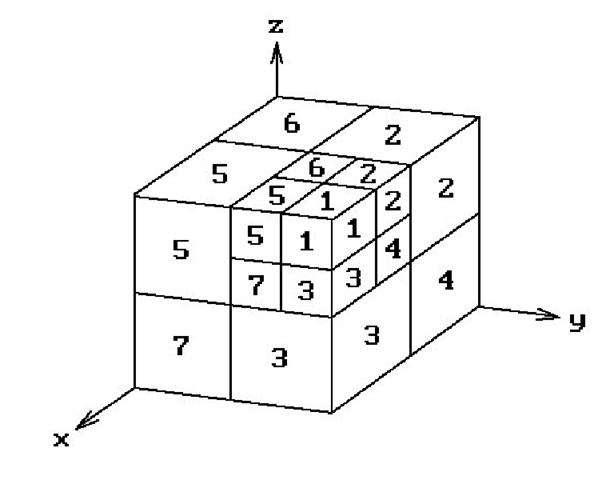
Because of the regular geometric structure underlying octrees, it is fairly easy to devise list priority visible surface algorithms for objects represented in this way if one is using a parallel projection. One lists the voxels in a back-to-front order. For example, consider Figure 7.11 and assume that the camera is in the first octant looking toward the origin. In that case, the sequence 8, 7, 4, 6, 5, 2, 3, 1 is one order in which to list the voxels so that no voxel in the list will ever be obscured by a voxel appearing earlier in the list. As each voxel is subdivided, we would use the same order for the new subdivided voxels.
Figure 7.11. Determining a back-to-front order for voxels.
Assuming that the voxel faces are parallel to the coordinate planes, it is straightforward to define a back-to-front order for the voxels for an arbitrary orthographic projection based simply on knowing into which of the eight octants the view plane normal is pointing. This can be generalized to an arbitrary parallel projection, not just orthographic projections. Having decided on a back-to-front order of the voxels (there is more than one), one then simply writes them to the frame buffer in that order like in the painter’s algorithm. For more details and references to papers see [FVFH90] and [Roge98].
One has to define discrete 3d rays first, which is done in Section 10.4.1.
Curved Surface Algorithms
One of the earliest curved surface visible surface algorithms is Catmull’s z-buffer algorithm described in [Catm75]. It recursively subdivided surface patches until they covered a single pixel and then updated the z-buffer appropriately. In this section we describe a scan line approach that is due to Blinn ([Blin81]). Before we start, however, we need to point out that curved surface algorithms like Blinn’s are hardly, if ever, used anymore. Nowadays, one simply generates a sufficiently close polygonal approximation to the surface and displays those polygons.High-performance graphics systems now have hardware support to make this feasible. Nevertheless, it is worthwhile discussing Blinn’s algorithm anyway because it brings out some interesting aspects of curved surfaces.
Let us begin with a review of the polygonal case. The top level scan line algorithm was:
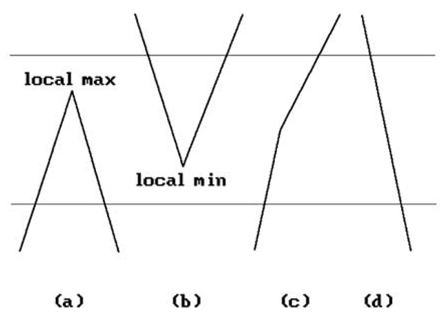
Figure 7.12. Basic cases to watch for in scan line algorithms.
Of course one had to make this practical using "coherence." We made incremental computations and had "active edge lists." Figure 7.12 shows the basic cases for which we had to watch out as we moved from scan line to scan line. We did various sorts to speed things up.
As we pass to curved surfaces we need to handle new cases. Assume that the surface is parameterized by a function
We need to look at level curves. Again assuming an orthogonal projection with the y-axis corresponding to scan lines, these level curves are defined by equations
In the linear case all the geometric information was contained in the edges and these could be represented by their endpoints. Now this is not enough because of "silhouettes." A silhouette is formed by points where the normal to the surface is orthogonal to the z-axis (or line of sight for a nonorthogonal view).
Let us keep track of points on level curves that are endpoints on patches or silhouettes. We shall do this by keeping track of their parameter values (u,v) and update them as we move down the scan lines. This is an important point, namely, that as maintaining "edge trackers." The questions that need to be asked are: How are “edge trackers" defined? How do they get their edges? How do edges appear/disappear
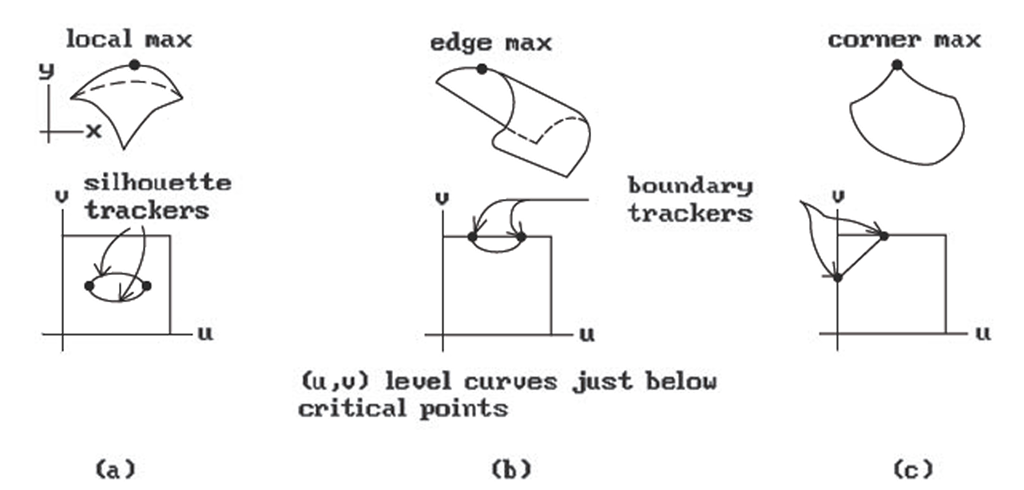
Figure 7.13. Some boundary tracker cases.
one works here in parameter space rather than the corresponding points in 3-space. Blinn refers to this tracking process ?
To see how edges are created, assume that all the critical points and maxima and minima of f have been found. Figure 7.13 shows some possible cases. The type of edges that are created depends on the type of critical point. In case (a) we have a strict local maximum. From that we get an elliptical intersection and two silhouette trackers. In case (b) we have an edge maximum with a parabolic intersection for two boundary trackers. In case (c) there is a comer maximum that basically gives us a linear intersection for two boundary trackers. In all these cases, initial (u,v) values must be found. These are then updated using a Newton-Raphson method where possible. This works fine in case (c) using the corner as a starting point. In cases (a) and (b) we cannot update with the Newton-Raphson method because the derivative vanishes. Instead, one uses the second derivative of f to locally approximate the level curve of f at the next scan line by a parabola or ellipse. This approximation of the level curve is used as an initial guess at (u,v).
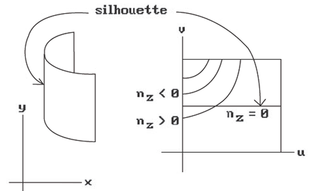
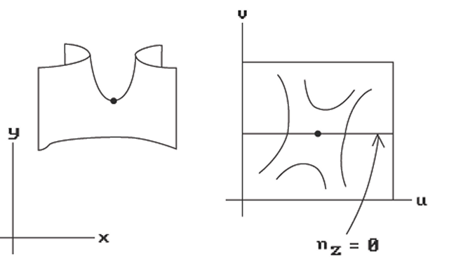
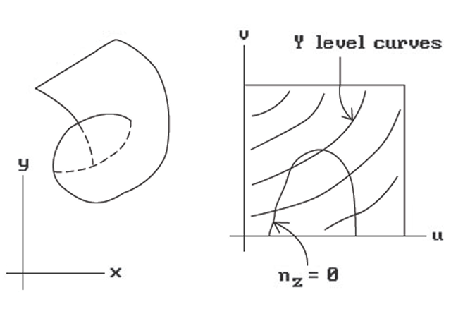
Unfortunately, there are all kinds of things that can happen in the curved surface case other than “standard" maxima and minima. Figure 7.14 shows a “folded edge." This is detected by checking the sign of the z- component of the normal, denoted by nz, of each boundary tracker. If it changes from one scan line to the next, then we have this case. What we have to do is to create a new silhouette tracker using the z-coordinate of the boundary edge tracker as an initial guess. Figure 7.15 shows a saddle point. Such points cause the creation of a new silhouette tracker.
When it comes to deleting edge trackers, there are two events for which we have to watch:
(a) when passing a local minimum or
(b) when a silhouette leaves at a boundary.
Figure 7.14. Checking for a folded edge.
Figure 7.15. Checking for a saddle point.
One deals with (a) by maintaining a list of local minima. Then when one updates the Y-scan, one checks against this list but keep in mind that
(1) The list gives the value in u-v space and we need to find the corresponding point on the edge tracker, that is the scan line.
(2) The numerical operations may fail to converge near such points. Therefore, use a modified Newton-Raphson iteration and discard those points which do not converge.
With regard to (b), we have to keep checking u and v to see if they still lie in [0,1] as we update the silhouette tracker. If either value does not, then delete the tracker.
When moving along a scan line from left to right one needs to maintain a list of active intersection points. These are obtained from the cross-section curves in the x-z plane. The intersections should be kept sorted by their x value. New points enter and leave this list at boundary edges and silhouettes. One updates their value by a two-variable Newton-Raphson method applied to the equations
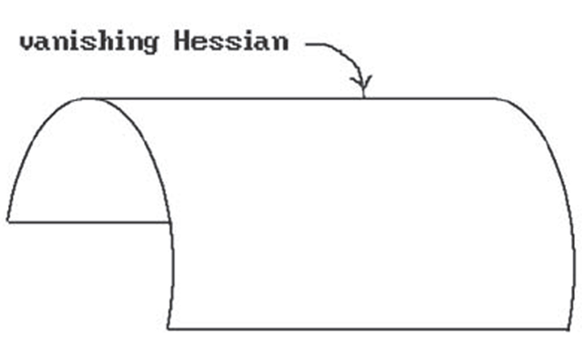
Figure 7.16. A vanishing Hessian case.
Figure 7.17. A curtain fold example.
We have outlined the main idea behind Blinn’s approach, but to implement it one has to overcome a number of special problem cases often caused by denominators vanishing in certain expressions. Some examples of these are:
Vanishing Hessians: See Figure 7.16. Here we need four edge trackers below a maximum, rather than two. The hard part is to decide when such a phenomena occurs.
Curtain folds: See Figure 7.17. Here nz becomes tangent to a y-level curve. One would need another pre-scan for such points, but Blinn avoids this via a heuristic.
Singularities intersecting singularities: This is a very general problem. An example of this is where a strict local maximum lies on the boundary of a patch.
With regard to the speed of the algorithm, Blinn found that the average number of iterations needed for the convergence of edge trackers was about 2.5. He was able to improve this substantially by extrapolating in the u-v space: He saved the (u,v) value from the previous scan line and used for an initial guess an extrapolation of the previous two values. This reduced the average number of iterations to less than 1.
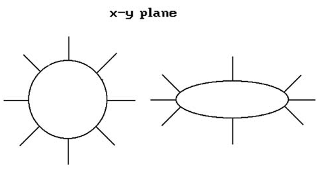
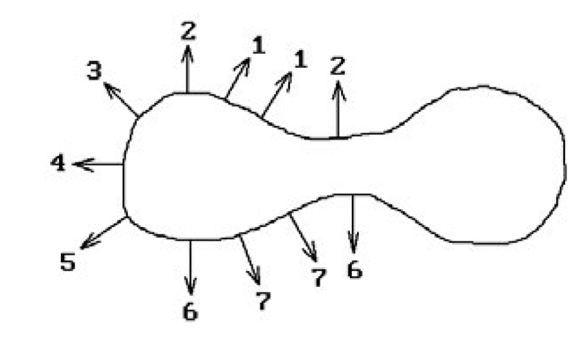
To speed the x-scan Blinn found intersections by choosing a sample of points and interpolating. This amounted to approximating level curves via polygonal lines. The sample points were chosen by spacing them equally according to the angle of the normal to the curve. Note that this clusters at places of high curvature. See Figure 7.18.
Figure 7.18. Using curve normals for subdivision.
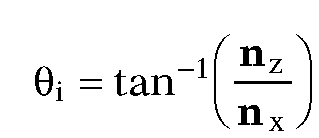
The computation for finding the points was similar to the way that silhouettes are found, except that now one allows other angles. More precisely, one solves
or
We can precompute the values sin![]() This gives a whole new set of edge trackers. All the edge trackers above must be linked together appropriately to get a polygonal approximation to the intersection curve. Links are created as we pass critical points. When we pass saddle points we get breaks that must be repaired by "sideways" iteration. One moves along level curves of constant y but changing Θ. A new edge tracker is created.
This gives a whole new set of edge trackers. All the edge trackers above must be linked together appropriately to get a polygonal approximation to the intersection curve. Links are created as we pass critical points. When we pass saddle points we get breaks that must be repaired by "sideways" iteration. One moves along level curves of constant y but changing Θ. A new edge tracker is created.
Using this approximation, level curves at a scan line are a chain of edge trackers that can be specified by an index into a table of sines and cosines. The angle rotates and we would expect that the index changes by 1 as we move from one edge tracker to the next (except obviously when we pass from the end of the table to the beginning). There is one other case however. The angle Θ can have local maxima or minima as we move around. See Figure 7.19. This occurs at inflection points of cross-section curves. Mathematically, if v is the tangent to the level curve, the directional derivative of Θ in the direction v vanishes: DVq = 0. We need to create trackers to follow this function.
The x-sampling described above sometimes made the polygonal nature of the approximation obvious in the output. Nevertheless it seemed to be reasonably good and did not use an excessive amount of time to compute. For smooth shading, most of the time was spent in the y-iteration. Blinn’s approach made surfaces look better than if one had used a polygonal approximation to them.
A Summary of the Blinn Algorithm. It is a scan line algorithm that generalizes polygon visible surface algorithms and involves solving equations determined by various geometric features, such as
Figure 7.19. An inflection point case with angle trackers.
|
Feature |
Equations |
|
|
boundary curves of patches |
 |
|
 |
 |
|
|
silhouette edges |
 |
 |
|
local maxima or minima |
 |
 |
|
segments of x-scan |
 |
 |
The equations are solved by making initial guesses and then using a Newton-Raphson iteration. One has a current active segment lists with segments being created and deleted and one sorts to find visible points. Blinn used heuristics to handle the many problems that arose.
We mention several other curved surface algorithms:
The Whitted Algorithm ([LCWB80]). This algorithm generalized the handling of surface patches bounded by straight lines to the case where boundaries are cubics. It avoided the problem of polygonal silhouettes but had problems with internal silhouettes and numerical techniques.
The Carpenter-Lane ([LCWB80]) and Clark ([Clar79]) Algorithms. These algorithms, like Catmull’s algorithm ([Catm75]), use a subdivision technique that ends up subdividing patches until they are flat enough so that they can be approximated by planar polygons. The polygons are then scan converted using a standard approach. The approximation is as good as the view requires but not a priori. Unlike Catmull’s algorithm, these are scan line algorithms. A problem that the algorithms have to worry about is that cracks can appear in the image if adjacent patches are not approximated carefully.
Blinn’s algorithm is actually more general than either the Whitted or Carpenter-Lane algorithms.
Adding Antialiasing
So far in our discussion of visible surface algorithms, we have only touched on the aliasing issue. In fact, these algorithms often have antialiasing techniques built into them. Some general references that have a lot more material on antialiasing methods than we shall mention here are [MagT87], [FVFH90], [WatW92], and [Roge98].
We already mentioned antialiasing lines and polygons in Section 2.6. Antialiasing algorithms are incorporated into image precision algorithms, such as the Warnock algorithm, by a supersampling type approach. One subdivides to below a pixel and averages the subpixel values.
Early antialiasing efforts in scan line algorithms ([Crow77a], [Catm78]) led to the A-buffer algorithm that is used for antialiasing in Z-buffer algorithms. This algorithm originated with [Carp84] and was subsequently improved by [AbWW85]. A pixel is again assumed to have area, but rather than making complicated geometric clipping computations on this area one associates a bitmask to the pixel (Carpenter used a 4 x 8 bitmask) and one does the clipping via Boolean operations on the bits, which is much faster. The bitmasks are used in conjunction with a z-ordering of the polygon pieces. An edge fill scan conversion algorithm is used to enter the edges of the polygon pieces into the bitmask. The bitmasks are initialized to 0 and in the end have a certain number of 1′s. A simple counting of the number of 1′s determines the percentage of area of the polygon piece that is used to determine its contribution to the shade associated to the pixel. See [MagT87], [WatW92], or [Roge98].
For antialiasing in ray tracing, see Section 10.2.
Conclusions
We finish the topic with some observations on visible surface algorithms. To begin with, note the importance of coherence. Basically, one thinks of a picture as consisting of regions all of whose pixels have the same value. Once we have the value of a pixel for a region, then we keep setting all adjacent pixels to the same value until we run into one of those "few" boundaries between regions where a change takes place. Below is a sampling of some different types of coherence guidelines when dealing with linear polyhedra.
Edge coherence: The visibility of an edge changes only when it crosses another edge. Therefore, we can create a list of edge segments without intersections and need only check one point per segment.
Face coherence: A face is often small compared to the whole scene. Therefore, usually the whole face is visible if one point of it is.
Object coherence: The use of bounding objects is a form of coherence.
Depth coherence: Different surfaces are usually well separated in depth.
Scan line coherence: Segments visible on one line are likely to be visible on the next.
Frame coherence: Images do not change much from frame to frame.
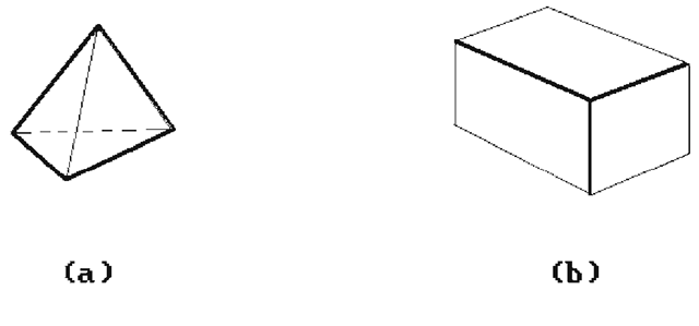
Geometric coherence: The possible visible/invisible configurations at any vertex are limited. For example, in a convex object the outside lines are visible (Figure 7.20(a)) as are all the edges surrounding a vertex (Figure 7.20(b)).
Figure 7.20. Examples of geometric coherence.
Curved objects satisfy similar types of coherence.
Visible surface determination algorithms need to be evaluated in the context of the whole rendering algorithm. There is no “best” such algorithm. Differences in algorithms stem from different requirements: different scenes, different complexity of output.In general though, image space algorithms seem to be the most popular. In fact, it is fair to say that Z-buffer algorithms, which are extremely simple and versatile, are the de facto standard in high performance graphics system because the price of memory is no longer such a problem. Furthermore, as mentioned earlier, because these systems typically have hardware support for fast display of polygons, all surfaces, including curved ones, are treated as collections of polygons. Many of the mathematical complications in algorithms like Blinn’s are thereby avoided. Of course, having a high-speed system is now more important than ever because of the large number of polygons with which one has to deal.
The table below summarizes normalized speed results from Table VII in [SuSS74]:
|
Number of facets in the scene |
|||
|
Algorithm |
100 2500 |
60000 |
|
|
Schumacker |
30 |
179 |
1215 |
|
Newell-Newell-Sancha |
1 |
10 |
507 |
|
Warnock |
11 |
64 |
307 |
|
Z-buffer |
54 |
54 |
54 |
|
Watkins |
3 |
21 |
457 |
In the table we have normalized the Newell-Newell-Sancha algorithm to 1. The numbers are estimates only though and should mainly be used for comparison purposes. Small differences are inconclusive and only orders of magnitude are significant.
Depth sorting and scan line algorithms are good if there are only a small number of surfaces (up to several thousand). Scan line algorithms take advantage of coherence between successive scan lines and of span coherence within a scan line. They reduce a three-dimensional problem to a two-dimensional one. One danger though is that very narrow polygons can fall between scan lines. In general, depth sorting is good if the scene is spread out in depth (relative overlap in z-direction) and scan line or area-subdividing algorithms are good if surfaces are separated horizontally or vertically.
For scenes with very large numbers of objects, z-buffer methods or methods designed for objects encoded as octrees are good because their complexity is independent of the number of surfaces.
Sorting is an extremely important part in all the algorithms we discussed. In a sense the real difference between all the algorithms is just in the way they sort. The sorting technique chosen should match the statistical properties of the data being sorted. See [SuSS74] for how sorting affects algorithms.
