Introduction
After modeling the geometry, the next basic step in a realistic rendering of a scene from a given viewpoint involves determining those surface patches that will be visible from this viewpoint. This is the visible surface determination problem. In the past this was called the hidden surface removal problem, but the terminology is beginning to change in order to emphasize the positive rather than the negative aspect of the problem. Many visible surface determination algorithms have been developed over the years. This topic describes several well-known such algorithms. Although the emphasis is on algorithms for linear polyhedra, we also discuss the additional complexities encountered in curved object cases. The ray tracing approach to visible surface determination, where one simply sends out rays from the camera (or eye) and checks which surface is hit first.
An excellent overview of some of the very early algorithms can be found in [SuSS74]. In general, visible surface determination algorithms can be classified as belonging to one of three types: object precision, image precision, or list priority. (We shall follow [FVFH90] and use the more descriptive term "precision” rather than the older term "space,” as in "object precision algorithm” rather than “object space algorithm”.)
Object precision algorithms are of the form
whereas image precision algorithms are of the form
Both types of algorithms do all their computations to the same precision in which the objects were defined. The main difference between them is that the former accurately compute all the visible parts of the world whereas the latter only determine visibility in a sampled number of directions. The complexity of image precision algorithms depends on the resolution of the screen, whereas the complexity of object precision algorithms does not (except at the last stage when regions have to be scan converted). In that sense, with the former one has to worry about aliasing. Pure object precision algorithms were used only in the early days of graphics, mainly on vector graphics devices. Given a raster graphics device it is only natural to use the discreteness of the pixels to help make the algorithm efficient.
Ray tracing captures the essence of image precision algorithms, which can be further subdivided into whether they deal with areas or points (area versus point sampling). The Warnock algorithm is an example of the former. The Z-buffer algorithm, the Watkins algorithm, and ray tracing are examples of the latter.
List priority algorithms fall somewhere in between object and image precision algorithms. They differ from pure image precision algorithms in that they precompute, in object space, a visibility ordering before scan converting objects to image space in a simple back-to-front order. Obtaining such an ordering may involve splitting objects. The Schumacker, Newell-Newell-Sancha, and BSP tree algorithm are examples of this type of algorithm.
Each algorithm described in this topic was selected with certain considerations in mind, which were:
(1) It is currently an acceptable approach in its intended application.
(2) The algorithm was interesting for historical reasons and easy to describe.
(3) It involved the use of some interesting techniques, even though it itself is no longer a recommended method.
This led to the following list categorized by (1)-(3) above:
|
Algorithm |
Category |
Comments |
|
Schumacker-Brand-Gilliland-Sharp |
(2) |
The first list priority algorithm. |
|
Newell-Newell-Sancha |
(2), (3) |
A depth sort list priority algorithm. |
|
The BSP algorithm |
(1), (2) |
A list priority algorithm. |
|
Warnock |
(2), (3) |
An area subdivision image precision algorithm. |
|
Weiler-Atherton |
(2), (3) |
A more sophisticated area subdivision algorithm. |
|
The Z-buffer algorithm |
(1) |
The algorithm used originally on high-end graphics work stations but now in most graphics systems. |
|
Watkins |
(1), (2) |
A scan line algorithm that is still worthy of consideration in certain applications because it is much faster than a ray-tracing-type algorithm. |
|
Ray tracing |
(1) |
The approach used in conjunction with radiosity methods if one wants the highest quality realistic images. It is discussed at length in Chapter 10. |
|
Octree |
(1) |
A list priority algorithm useful for volume rendering |
|
The Blinn curved surface algorithm |
(2), (3) |
The algorithms above, except for the ray-tracing algorithm, will be discussed in Sections 7.3-7.10. Section 7.2 will describe a preprocessing step called back face removal, which is easy to carry out and saves the algorithms a lot of needless work, but can also be used all by itself to provide some rudimentary realism to scenes. When we discuss the visible surface determination algorithms, the reader needs to be aware about one assumption that is made because it is convenient. Unless explicitly stated otherwise, we shall assume the following:
The orthogonal projection assumption: We assume that the world has been transformed into a coordinate system where the eye is at infinity, so that the projection to the view plane is an orthogonal projection (rather than a central projection) and corresponds to simply dropping the z-coordinate.
Finally, it should be mentioned that there are also visible line determination or hidden line removal algorithms. These algorithms are used mainly in the context of wireframe displays. Every visible surface determination algorithm can be modified into a visible line determination algorithm, but not vice versa. For an example of this see [PokG89]. The earliest visible line determination algorithm was developed by Roberts in [Robe63]. It assumed all lines came from edges of convex polyhedra. First, back edges were removed. (A back edge is a common edge of two back faces.) Each remaining edge was then checked against all the polyhedra that might obscure it. [Roge98] describes this algorithm in great detail. A more general purpose visible line determination algorithm was described by Appel in [Appe67]. Appel introduced a notion of the quantitative invisibility of a point, which was the number of front-facing polygons that obscured the point. A point was visible if and only if its quantitative invisibility was zero. Visible line determination lost its importance as computers became more powerful.
Back Face Elimination
The simplest way to render in a geometric modeling program is to display the world in wireframe mode. Such displays might be quite adequate for the task at hand and they have the added advantage that they are fast. An extremely easy way to make them look more realistic is to eliminate edges common to "back faces."
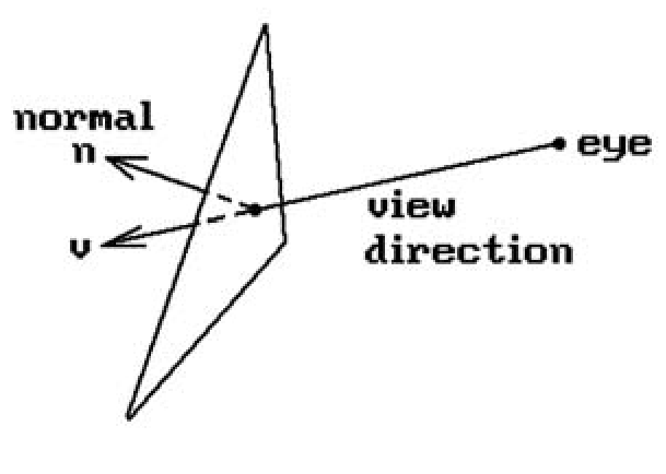
A back face of a solid object is a face that is facing "away from" the camera. To explain what this means and derive a test for it we need to look at normal vectors. Recall the discussion in Section 6.4. The faces of a solid have a natural outward-pointing normal vector associated to them. On the other hand, a choice of a normal vector for a face is equivalent to having an orientation for the face. Therefore, a general definition for a back face is the following (see Figure 7.1):
Definition. An oriented face is called a back face with respect to a vector v (typically the view direction of a camera) if the angle between its normal vector n and v is between 0 and 90 degrees. Mathematically, this simply means that n · v > 0. If n · v < 0, then it is called a front face for v.
This definition of back face also handles the case of faces in an arbitrary oriented surface patch that may not be the boundary of a solid, such as the upper hemisphere of the unit sphere or a bicubic patch.
Removing edges on the back faces in wireframe mode works pretty well on boundaries of solids, such as a sphere. On the other hand, some viewers may not be happy with the result in other cases. For example, if one looks diagonally down on a cylindrical surface, back face removal would only show half of it even though the back part would actually be "visible" from the viewpoint. For that reason, a modeling program should have the ability to flag a face as "two-sided," meaning that it should be treated as a "front" face no matter where the viewpoint is.
Finally, it is important to realize that back face removal is based on a local decision. It does not guarantee that the faces that are left are in fact visible. They might be obscured by some other object or even another part of the same object if it is not convex. Therefore, back face removal in no way saves us from a subsequent visible surface determination algorithm. If one wants to display only visible surfaces, one will still basically have to check each face against every other face to see if one obscures the other. What it does do however is cut down the number of faces that have to be looked at by a factor of two on the average, which is a substantial savings, and so visible surface determination algorithms usually have this built in as a preprocessing
Figure 7.1. Defining a back face.
The Schumacker List Priority Algorithm
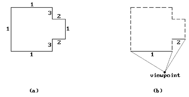
The original list priority algorithm is due to [SBGS69]. Its major contribution was the idea that faces of objects can sometimes be given a priory ordering from which their visibility can be computed independently of the viewpoint. Figure 7.2 shows an example of this. Figure 7.2(a) shows possible priority numbers for the faces. Figure 7.2(b) shows how one uses these numbers. Once an actual viewpoint is specified, one eliminates back faces (shown with dotted lines) and then uses the priority numbers on the remaining faces to tell which face is in “front” of another one. More accurately, if one face has a lower priority number than another one, then this means that the second will never obscure the first. In the figure, we would conclude that the face with priority number 2 does not obscure the face with priority number 1. Given the priority numbers we can then use the so-called painter’s algorithm, Algorithm 7.3.1, to draw the scene. The painter’s algorithm gets its name from the way a painter paints an oil painting. As the brush draws over other paint it covers it up.
Of course, the priority numbering that Schumacker was looking for does not always exist for the whole world. One can, however, divide the world into prio-ritizable clusters, that is, collections of faces within which one can assign priority numbers to each face with the meaning above. These clusters will then themselves have to be prioritized. One big problem with Schumacker’s approach was that too much had to be done by hand, but it was useful in situations where the objects in the scene did not change much and only the viewpoint changed, as, for example, in Schumacker’s own application to a flight simulation program.
Figure 7.2. A priority ordering for faces.
Algorithm 7.3.1. The painter’s algorithm.
Newell-Newell-Sancha Depth Sorting
The Newell-Newell-Sancha visible surface algorithm ([NeNS72]) is an early list priority algorithm that sorts objects by depth and then uses a painter’s algorithm to display them. One important difference between it and the Schumacker algorithm is that it computes the depth ordering on the fly and does not rely on an a priori ordering like the Schumacker algorithm. For that reason it is a more versatile algorithm. It introduced some interesting ideas on how to obtain a depth ordering.
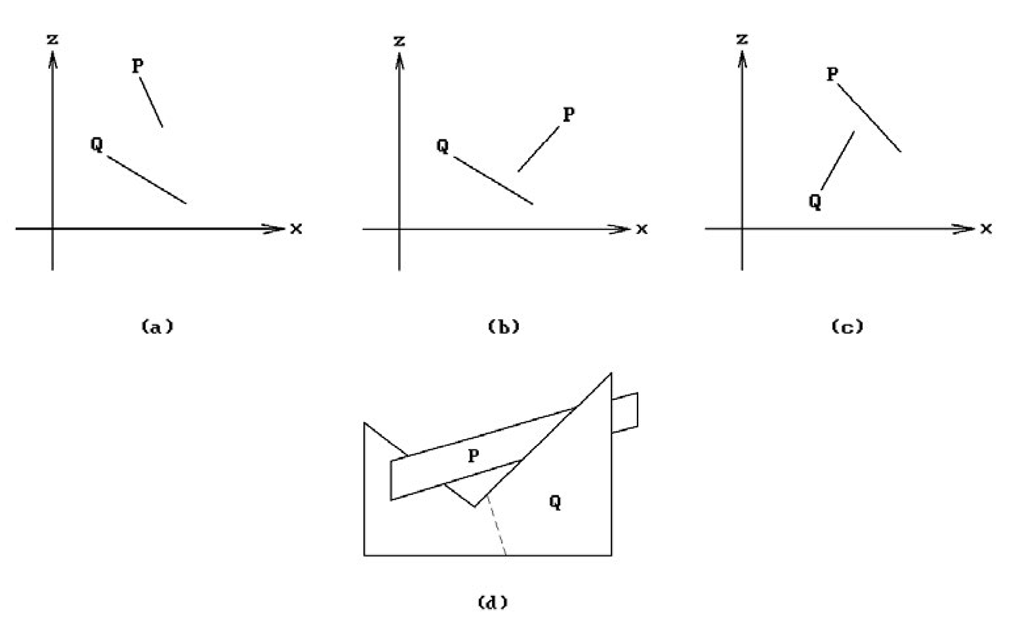
The Newell algorithm does an initial crude ordering of the polygon faces of objects based on the z-value of that vertex of a face that is furthest from the viewer. Next, starting with the last polygon P in the list (the one furthest from the viewer) and the next to the last polygon Q, one checks if P can be safely written to the frame buffer by asking whether P and Q separated by depth, that is, whether
If yes, then P can never obscure any part of Q and we can write P to the frame buffer. See Figure 7.3(a). If no, then one considers the set {Q} of polygons that overlap P in depth.
Figure 7.3. Some relative positions of faces.
Although there is this overlap in z, P may in fact not obscure any part of any of the Qs, and so the algorithm performs a series of tests, ordered by complexity. These tests involve answering the following questions:
(1) Can one separate P and the Qs in x?
(2) Can one separate P and the Qs in y?
(3) Is P on the farther side of the Qs? See Figure 7.3(b).
(4) Are the Qs on the near side of P? See Figure 7.3(c).
(5) Do P and the Qs project to disjoint sets?
Test (5) is clearly the most complicated and the hope is that one does not have to perform it very often. If the answer to all these tests is "no," then one swaps P with a Q and repeats the tests. One has to mark the Q to prevent getting into an infinite loop. An attempt to swap an element already swapped at a previous stage implies that one has encountered a "cyclical overlap." An example of this is shown in Figure 7.3(d). In that case one would cut Q at the dotted line and replace the old Q with the two parts. Eventually one would be able to write the polygons to the frame buffer.
The Newell algorithm handled transparency effects by overwriting the frame buffer only partially. However, aside from the historical interest, the interesting aspect of the algorithm comes from tests (1)-(4), which can be useful in other situations.
The BSP Algorithm
The Binary Space Partitioning (BSP) algorithm ([FuKN80] and [FuAG83]) is a visible surface algorithm that improved on Schumacker’s work by automating the division into clusters. The basic BSP algorithm consists of two steps:
(1) A one-time preprocessing step that converts an input polygon list into a binary tree structure called a BSP tree
(2) A traversal algorithm that traverses this tree and outputs the polygons to the frame buffer in a back-to-front order
A key idea here (like in Schumacker’s work) is that of a separating plane. The main condition that this plane has to satisfy is that no polygon on the viewpoint side of the plane can be obstructed by a polygon on the other side. To construct the BSP tree, one proceeds as follows:
(1) Select any polygon P from the current list of polygons and place it at root of tree.
(2) Each remaining polygon in the list is then tested to see on which side of P it lies. If it lies on the same side as the viewpoint one puts it in the left (or "front") subtree list, otherwise one puts it in the right (or "back") subtree list. If a polygon straddles Ps plane, divide it along that plane and put each of the pieces in the appropriate subtree list.
(3) Repeat this procedure recursively on the two subtree lists.
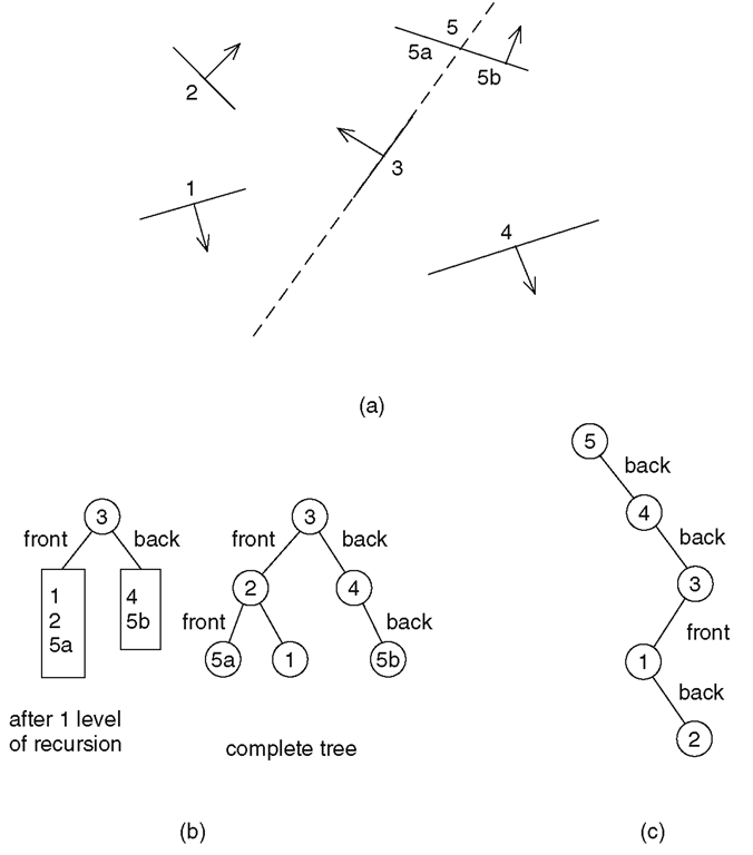
Figure 7.4. A BSP example.
Consider the example shown in Figure 7.4. There are five polygons numbered from 1 to 5 in Figure 7.4(a). The arrows are supposed to indicate the side containing the viewpoint. (In this example, the chosen directions do not correspond to a possible situation.) We assume that polygon 3 is the one chosen first, then 2 and finally 4. The stages of the BSP tree are shown in Figure 7.4(b). Note that choice of polygons can greatly influence the outcome. Figure 7.4(c) shows the tree that we would get if the polygons were chosen in the following order 5, 4, 3, 1, and 2.
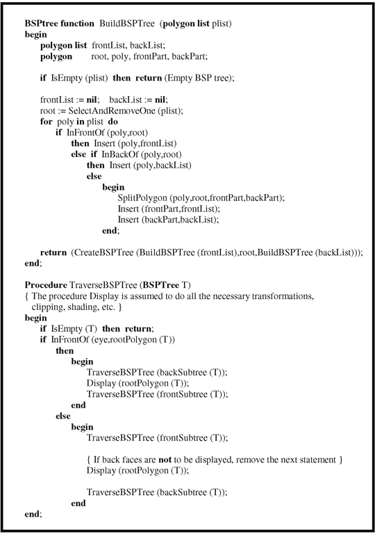
Once the BSP tree is generated, it is easy to generate the view by traversing the tree in in-order fashion. At each node of the tree determine whether the eye is in front or in back of the current root polygon. Traverse the opposite side of the tree, output the root polygon to the frame buffer, and then traverse the remaining side.
Algorithm 7.5.1 is a more precise description of how the BSP tree is built and traversed. It was originally feared that the BSP tree would be significantly larger than the input polygon list, but this did not turn out to be the case in practice. To cut down on the number of polygons that are split, the following heuristic was used: Select that polygon to be the root of the next subtree that cuts the fewest other polygons. It was discovered that it was not necessary to look over all of the remaining polygons. Rather,it was sufficient to choose the best from a few chosen at random (five seemed to work well).
Algorithm 7.5.1. The BSP tree algorithm.
We have just described the original BSP algorithms. Variants have been developed since then. For example, Kaplan ([Kapl85]) chose his separating planes to be parallel to the coordinate planes of the reference coordinate system. Such an algorithm is sometimes called an orthogonal BSP algorithm. This property of separating planes can simplify computations, especially when objects have bounding boxes. We shall mention other BSP algorithms later on when discussing ray tracing in Section 10.2.
To summarize, the BSP algorithm is a good algorithm where the world model does not change much and only the viewpoint changes. Examples of such situations are flight simulators, architects walking through a house, and biochemists viewing complicated molecules. Chin ([Chin95]) describes an efficient way to implement and use BSP trees.


