Overview
This topic covers a number of applications that involve local properties of surfaces. Section 15.2 discusses some curvature-related topics. Sections 15.3-15.4 deal with geodesics on surfaces. We discuss algorithms for generating both smooth and discrete geodesics and then describe an application to filament winding and tape laying. Section 15.5 is on how one can drop curves onto surfaces, something that is important in robotic applications. Section 15.6 discusses a few blending topics.
Curvature
Curvature raises its head at many places in CAD and CAGD. It is important to fairing curves and surfaces. We have also seen it in the context of finding efficient polygonal representations for curves and surfaces. For example, if a parametric surface has many relatively flat spots, then using a polygonization of the surface that is obtained by evaluating points at a uniform grid in parameter space would be very wasteful. To minimize the space for the data structure one would want a relatively coarse subdivision for flat regions and only use a much finer subdivision at the more curved parts. Clearly, flatness is a function of curvature. This section presents a sample of the curvature topics that one finds in the literature by summarizing the findings of several technical papers that have been published on the subject. The interested reader can find other references in those papers.
To begin with, there is the notion of curvature itself. In the case of curves, there is really only one concept of curvature and computing it involves the second derivative of the curve. In the case of surfaces, the situation is not as simple because there are a number of different curvature related concepts. The most important is Gauss curvature, but principal and mean curvatures are also useful. To compute these one needs second order partial derivatives.
We consider curves first. The fairness of a curve is defined in terms of curvature. See Section 11.12. Typically one seeks curves whose curvature functions are appropriately piecewise monotone. Sapidis ([Sapi92]) describes a simple geometric condition so that a quadratic Bezier curve segment has a monotone curvature function. It is furthermore shown how to move the middle control point of that segment to correct any bad curvature plot it may have initially.
Just because we have an approximation that is within a given tolerance of an object does not mean that the shape of the object has been approximated very well. A curve that wiggles about a straight line would not be a good approximation of the shape of the line. As was indicated in earlier topics, the choice of metric with respect to which an approximation is defined matters. Wolters and Farin ([WolF97]) describe a metric based on total curvature that does a better job in approximating shape.
Miura ([Miur00]) proposes a new type of curve whose curvature is easier to manipulate than that of the more traditional curves. The method is based on integrating tangent vectors, specifically unit tangent vectors. In order to make this easier for the user to define such vectors, the author’s system asks the user to pick points on the unit sphere in an interactive way. The selected vectors are interpolated by thinking of them as unit quaternions. This construction is the analog of the clothoid construction that has been used to manipulate plane curves in a way that controls curvature properties. Miura calls his curve a unit quaternion integral curve.
Next, consider surfaces. Krsek et al. ([KrLM98]) describe methods for computing curvature quantities from discrete data. The approach is to approximate the data by second order curves or surfaces. Higher orders did not seem to lead to much improvement. They describe various methods but analyze
The circle fitting method: This turns out to be the fastest.
The paraboloid fitting method: This is slower than the circle fitting method but more accurate on noisy data.
The Dupin cyclide method: This is the slowest but is usually more accurate than the other two methods.
Wollmann ([Woll00]) also tries to estimate curvature values for a discrete surface. The method is based on getting estimates to the curvature of curves and using Euler’s and Meusnier’s theorem.
Meek and Walton ([MeeW00]) analyze the accuracy of various approaches to the problem of getting approximations to surface normals and Gauss curvature given a surface defined by a set of discrete points. The assumption is that one has accurate data for a smooth surface such as one would get from sampling points on a real object. They analyzed the following methods for finding an approximation to the surface normal and/or the Gauss curvature at a point p:
(1) Fitting a quadratic surface to the given data near p and using its normal and Gauss curvature as approximations.
(2) Approximating the surface at p by a set of triangles incident to p and using various types of averages of their normals.
(3) Approximating the Gauss curvature at p by discretizing its definition based on the Gauss map where one thinks of it as a limit of the quotient of small areas containing p and the area of their images on the unit sphere.
(4) Approximating the Gauss curvature at p by means of the angle deficit method.
One surprising conclusion was that the popular method (4) is not always very accurate.
Andersson ([Ande93]) discusses how one could design a surface by modifying its curvature. This is carried out in terms of solutions to boundary value problems for partial differential equations.
Ye ([Ye96]) points out how a color-coded Gauss curvature map can be used to judge the fairness of a surface. A smoothly varying map is good and rapidly varying ones are bad. Ye answers the following question about the fairness of a surface where two patches meet:
Question: Can the curvature continuity between the patches be visualized by means of the Gauss curvature? Alternatively, if two patches are tangent-plane continuous along their common edge and they have the same Gaussian curvature along the common edge, are they curvature continuous there?
There is a similar question for mean curvature. Let denote the normal curvature at a point p of a curve C lying in surface S.
Definition. Let S1 and S2 be surfaces that are tangent-plane continuous along a curve C. The surfaces are said to be curvature continuous along C if for all curves C1 and C2 on S1 and S2, respectively, that meet and are tangent at a point p on C we have that![]()
Ye gives an answer to the question in terms of Dupin indicatrices, principal curvatures, and Gauss and mean curvatures. Mean curvatures turn out to be a better way to measure curvature continuity.
Kaklis and Ginnis ([KakG96]) address the problem of constructing shape-preserving C2 surfaces that interpolate point sets lying on parallel planes. Call the planar curves pi(u) interpolating the data of a given plane a skeletal line. We are basically looking for a skinning surface p(u,v) for the skeletal lines pi(u). Kaklis and Ginnis describe how one can get a skinning surface that has the property that if the curvature of adjacent curves pi(u) and pi+1(u) has the same sign over an interval [uj,uj+1], then the curvature of all the curves p(u,v), v e [vi,vi+1] also has the same sign over the interval [uj,uj+1].
Wolter and Tuohy ([WolT92]) describe how to compute curvatures for degenerate surface patches.
Other aspects of surfaces that are sometimes interesting are their lines of curvature. Analyzing these involves solving differential equations. See [BeFH86]. Lines of curvature are used to define principal patches.
Finally, is there a notion of curvature in the case of polygonal objects? Such a notion would be defined at vertices and would be a function involving the angle between adjacent edges for curves and the sum of the angles of the faces meeting at a vertex for surfaces.
Geodesics
Generating Smooth Geodesics
The mathematics of geodesics for surfaces in R3 is discussed in Section 9.10 in [AgoM05]. The mathematical definition of a geodesic is that it is a function (a parameterized curve) defined by second-order differential equations. This is what we shall mean by the term “geodesic,” but it is sometimes used more loosely, for example, to refer to the underlying set that is traced out by a geodesic. A common statement is that a straight line in the plane is a geodesic, but one needs to remember that a line can be parameterized in many ways and only some of those parameterizations would actually fulfill the mathematical definition of a geodesic. Two other definitions that are given sometimes (and that consider geodesics as sets rather than maps) are:
The Kinematic Definition. A geodesic is a curve traversed by a particle whose acceleration vector at a point lies in the plane spanned by the velocity vector and the normal to the surface at that point. There is no “side-to-side” acceleration. Any acceleration that there is, is used to keep the particle in the surface or to speed it up or slow it down in the direction of the path.
The Static Force Definition. On a convex surface, a curve is called a geodesic if a thread stretched along the path it traces out on the surface is in static equilibrium with respect to any sideways tension on it.
A true geodesic would satisfy both of these criteria. However, a geodesic in the kinematic or static force sense would not necessarily be a real geodesic since its acceleration vector might not be orthogonal to its velocity vector. Nevertheless, by Theorem 9.10.11 in [AgoM05] it does trace out a geodesic path.
Note. The boundary of a surface causes technical problems for the definition of a geodesic because one often needs derivatives to be defined in open neighborhoods of a point. To avoid such problems, we shall assume throughout this section that either our surfaces have no boundary or that all the curves being defined are well away from the boundary.
Consider a surface patch S in R3 parameterized by
Any curve in S can be expressed in the form
 where
where
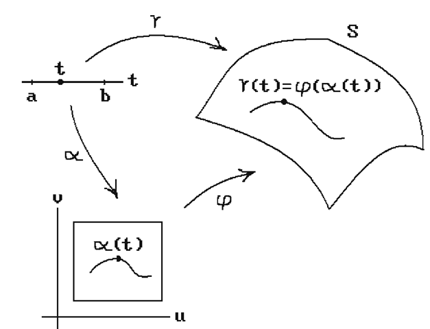
(If we were given γ first we could define See Figure 15.1. Let
Figure 15.1. Curve in parameterized surface.
and
We know that
form a basis for the tangent space at every point of the surface and
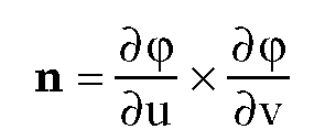
is a normal vector at those points. The chain rule implies that
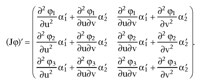
where is the Jacobian matrix for
![]() It follows that
It follows that
and
The condition on which makes the curve
 into a geodesic is that
This would lead to having to solve a second order differential equation for a. Instead, by introducing a new variable![]() one turns the system (15.3) into a system of first order differential equations, which is the usual preferred approach. See [PFTV86], for example, for ways to solve such systems of equations.
one turns the system (15.3) into a system of first order differential equations, which is the usual preferred approach. See [PFTV86], for example, for ways to solve such systems of equations.
Next, assume that we only want a geodesic in the kinematic or static force sense. In this case, equations (15.3) get replaced by the single equation
where
Of course, as was pointed out earlier, such a curve g(t) may not mathematically be a geodesic since g"(t) may not be a normal to the surface, but it will trace out a geodesic path. Now, assume that the curve a(t) above is an arc-length parameterization of a curve, so that |a’(t)| = 1. Let us parameterize the unit vectors a’(t) by the turning angle 0(t). In other words, write
It follows from (15.5) and the chain rule that
If we replace γ" in equation (15.4) by the right-hand side of equation (15.2) and also replace a" by the right hand side of equation (15.6), then one can solve for 0′(t). In fact, it is easy to show that solving (15.4) is equivalent to solving the following system of equations:
We shall return to this equation in Section 15.4.
Now what we have described so far are just local conditions for geodesics. The curves must satisfy the differential equations shown above in a neighborhood of any point through which they pass. Furthermore, there are of course many solutions to these equations and to get unique solutions one needs to specify additional constraints. The most common constraints, and the ones handled most easily with standard numerical techniques for solving differential equations, are initial conditions. Typical initial conditions would be a start point of the desired curve and a direction vector. However, this does not solve the problem of finding a shortest curve between two points because we would not know the initial direction of the curve. The shortest curve problem is a boundary value problem and much more difficult. A solution to the discrete version of this problem is described in the next section.
One area where one has to deal with geodesics is in the design and manufacture of composite materials. See Section 15.4 below. In this case one wants to generate geodesics given a start point and an initial direction. A common approach is to tes-sellate the surface and generate geodesics on the resulting polygonal surface. The paper [KSHS03] describes differential equations for a geodesic obtained from a variational approach and compares the numeric solution to these equations to the discrete geodesics one can generate on the approximating polygonal surface using two different algorithms. It turns out that the deviation of the discrete geodesics from the smooth geodesic is not always proportional to the error caused by the tessellation but depends also on the complexity of the surface.
We finish this section with an example. Unfortunately, just as very few curves have a simple formula for their length, very few geodesics have a simple formula. Nevertheless, the following may help the reader understand the mathematics.
Example. Consider the paraboloid of revolution S defined by the equation
and parameterization
We want to compute the equations that define the geodesics for this surface.
Solution. Let be a curve in the domain of φ. First of all, observe
that
so that
It follows from equation (15.3) that the geodesics of S are defined by curves a(t) satisfying
We shall not solve that system of differential equations, but will show that certain longitudinal curves (meridians) are geodesics in the kinematic sense.
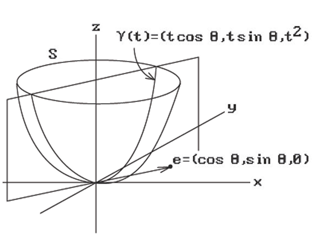
Let![]() be a fixed unit vector in the plane and consider the curve
be a fixed unit vector in the plane and consider the curve
The curve traces out the intersection of the vertical plane through the origin and e with our surface S. See Figure 15.2. It is easy to check that
Now,
Figure 15.2. Longitudinal curves that are kinematic geodesics.
and
is a kinematic geodesic (but not a geodesic since  is not a normal to the surface).


