Global Geometric Modeling Topics Part 6

Skinning

Sections 13.4.3 and 14.6 dealt with what might be called finding level curves of a given surface. This section turns the problem around.

Definition. A skinning surface for a sequence of sets 1is  a surface S satisfying

(1)    S interpolates the sets, and

(2)    there is a continuous functionand    real numbers

The process of finding such a surface is called skinning. In practice, the sets Ci consist of one or more curves, in which case they are sometimes called skinning curves.

In many cases, skinning is just a more recent term for lofting. Condition (2) of a skinning surface is simply trying to capture the intent that the curves C should be contours or level curves of the surface with respect to a function. Some skinning algorithms may at times produce self-intersecting surfaces, but that would be an undesirable “feature” of the algorithm. A common case for the curves is where they are planar and correspond to parallel cross-sections of a surface. It is easy to imagine though how complicated things might get if one is given an arbitrary collection of curves.

Of course, like in all interpolation problems, one wants more from the skinning surface S than that it interpolates the curves. Specifically, some properties that one wants S to satisfy are:

(1)    the shape of the surface should match the shape suggested by the curves and it should not have any unnecessary wiggles.

(2)    The surface should be smooth if all the curves are.

(3)    The algorithm for getting S should be affinely invariant, meaning that if the curves are moved by an affine transformation T, then the algorithm applied to the new curves T(Q) should produce T(S).

Skinning algorithms have been defined in two quite different contexts, a polygonal and a smooth one. The polygonal case, which is often the harder one, is where the curves are polygonal and we are looking for a faceted S. The smooth case is where the curves are smooth parametric curves and one wants a smooth parameterization for S. This section will only touch on a few aspects of the skinning problem. Two papers that have numerous references to work on this subject are [MeSS92] and [ParK96].

We consider the polygonal case of the skinning problem first. Meyers et al. ([MeSS92]) break this problem into four subproblems:

The correspondence problem: One has to determine a correspondence between closed curves of adjacent contours. This defines some crude topological properties of an object. For example, if two closed curves of one contour correspond to one closed curve on the next, this would indicate a saddle structure for the object. Clearly, the only hope for coming up with a reasonable answer to the correspondence problem is to assume that the contours of the skinning surface have been spaced close enough together so that simple heuristics will work.

The tiling problem: One has to determine a triangulation for the surface that is to span two adjacent contours. There is no unique triangulation, and so solutions to this problem try to optimize some function that measure the appropriateness of spanning surfaces. Many such “metrics” have been proposed. Each one has its problems.

The branching problem: If there is more than one closed curve on adjacent contours, then one may need to determine how two or more closed curves in one contour get merged into one closed curve in the next contour. This would typically also entail determining how parts on the closed curves of the first contour are related. The tiling problem is more complicated when there are branches. Early work on tiling tended to assume that there were no branches or expected a user to help out interactively.

The surface-fitting problem: After one has a tiling, one may want to fit a smooth surface to that tiling.

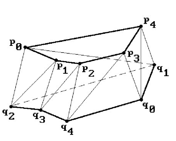
Let us look at a simple aspect of the tiling problem. Assume that two adjacent contours are defined by two closed polygonal curves with distinct vertices p0, p1, . . ., pm and q0, q1, . . ., qn, respectively. One would like a triangulation of the skinning surface S to look something like the surface shown in Figure 14.33, where m = n = 4. Now, in general, m and n are not equal, but the real problem is that one is not given any information about which point qj should connect to which point pi. For example, in Figure 14.33, how do we determine that q2 is the point that should be connected to po and p1? We certainly do not want to connect po and qo. It is not the case that there is no algorithm for finding the triangulated surface as shown in Figure 14.33. One could do an exhaustive search, but this would be prohibitively slow to carry out. The issue is finding an efficient algorithm. Fuchs et al. ([FuKU77]) reduced the problem to one of searching a toroidal graph. (A toroidal graph is a graph that can be embedded in a torus.) They used a “divide-and-conquer” technique along with an area-minimizing heuristic. A number of other approaches have been proposed using different heuristics. For such heuristics to work reasonably well, a common assumption is that the two curves satisfy some not unrealistic coherence condition. Basically, one assumes that the curves are closed, planar, coherent in size and shape, and mutually centered. By transforming the planar curves in a preprocessing stage one can always arrange it so that this is the case. [GanD82] describes an algorithm that runs in time O(m + n) using a heuristic that seems to work well in practice. [GanD82] also has references to other work. We refer the reader to that paper for details.

Figure 14.33. Skinning polygonal curves.

Meyers et al. ([MeSS92]) describe a skinning algorithm that handles the correspondence problem without requiring overlapping contours and generates a tiling even in the presence of relatively complex branching of contours and without adding new vertices. Park and Kim ([ParK96]) address the surface-fitting problem. They represent contour curves as cubic closed B-spline curves with a common knot vector and find an approximation to the skinning surface that is a C2 bicubic closed B-spline surface.

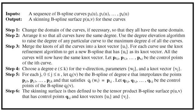
Next, we consider the skinning problem for a sequence of curves that are B-splines and describe the standard algorithm for creating a skinning B-spline surface. Algorithm 14.7.1 outlines the steps. Let

be the parameterization of the curve Cj after steps 1-3 in the algorithm. Piegl and Tiller ([PieT95]) suggest defining the parameters wj and knots vj in Step 4 as follows in order to match the chordal lengths:

Algorithm 14.7.1. A B-spline skinning algorithm.

where Li is the chord length of the polygonal curve with verticesand

There are problems with this approach.

(1)    The surface may not have the desired shape.

(2)    There may be lots of knots [uj] with some very close together causing potential numeric problems in applications that may use this data.

(3)    The surface may have self-intersections.

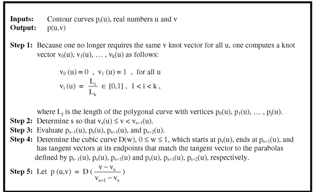
Part of the problems is caused by the fact that we had to choose the same knot vector for all the curves in the v-direction. In order to overcome some of these problems [FilB89] describes a skinning surface in a procedural way. This new method also does not require the curves to be B-splines. The steps to compute the parameterization p(u,v) at (u,v) are outlined in Algorithm 14.7.2. In practice, a cubic approximation to the function vi(u) simplified the computations and was found to be adequate.

Finally, we point out that skinning is really a special case of the more general surface reconstruction problem. We are given a set of scattered data points and want to fit a surface to those points. There is no time to go into this topic here, but we leave the reader with sample references for this and a related problem. In [BoiC00] the reconstructed surface is an implicitly defined smooth manifold. The paper [ACDL00] simplifies a previous algorithm and also proves that if the data came from a surface, then the construction is homeomorphic to the input surface. In [HuaM02] there is an algorithm for creating a combinatorial manifold mesh given some unorganized point samples from an existing object. A related two-dimensional problem is image reconstruction that involves fitting a continuous intensity surface through image samples and [YuMS01] describes an approach that does not depend on patch boundaries lining up with coordinate axes. These papers contain many additional references.

Computing Arc Length

Let

be a parametric curve. This section discusses algorithms that solve the following two problems:

Algorithm 14.7.2. A procedural skinning algorithm.

The Arc length problem: Compute the length L of p.

The Arc-length parameterization problem: Given s e [0,L], find the point q on the curve so that the part of the curve from p(a) to q has length s. In practice, the problem is one of finding u e [a,b], so that p(u) is that point.

By definition, the length L of the curve p in (14.21) is the limit of sums of the form

where the limit is taken over all partitionswhose norms go to zero. It follows thatwill be a good approximation to L provided that the polygonal curveis    a good approximation to the curve

p. Therefore, a quick and dirty    way to    estimating arc length is just    to    make a guess as to a    reasonable subdivisionand    then to use the valueWe can also get a quick estimate for q in the arc-length parameterization problem as follows:

(1)    Make a table of the lengths si    of the polygonal curve    defined    by the points

(2) Given s, find j so that

(3)  Setwhere    u    is the corresponding interpolated value inthat is,

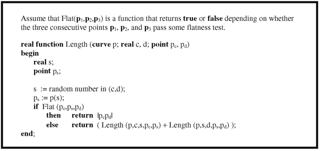
On the other hand, to get a more accurate values we must do more work. We start with the arc length problem. Our first good approximation to arc length based on equation (14.22) relies on getting a good polygonal approximation to the curve and then using the length of that polygonal curve. Any good polygonal approximation will work. One such is the de Figueiredo algorithm (Algorithm 14.3.1) described in Section 14.3, where one subdivides recursively until the curve is relatively flat according to some criterium. Algorithm 14.8.1 computes arc length based on the polygonal approximation that one gets from this.

Next, note that for smooth functions p(u) the sums L({uj}) in equation (14.22) are Riemann sums which converge to an integral. Specifically,

Therefore, another way to compute L is to use a known numerical approximation to integrals. Now sometimes one is in a situation where one has a fixed curve p(u) and one needs to answer multiple requests for arc lengths of different subarcs p([c,d]) of p(u). Guenter and Parent ([GueP90]) deal with this situation. The authors decided to use a Gaussian quadrature method for evaluating integrals because it is a particularly efficient integration method. They suggested that it is advantageous here to build a table of a certain number of precomputed arc length values in order to speed up the computation of other values.

For any c,d e [a,b], let GQ(c,d) denote the Gaussian quadrature approximation to the integral

Algorithm 14.8.1. Arc length based on polygonal approximation.

Note that since Gaussian quadrature is defined for functions defined over [-1,1], in order to use this method one must reparameterize the integral in (14.24) to

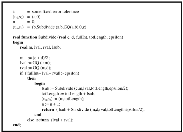
In [GueP90] one then builds a tableusing Algorithm 14.8.2. The form a partition of [a,b] and sj is a Gaussian quadrature approximation to

Using this table, if one wants L(a,u) one first finds the j so that and returns the value

Algorithm 14.8.2. Building a table for arc length computation.

 

Because u lies inthe computation forwill be fast.In general, for

anyis    computed asAlgorithm  14.8.2  is  an  adaptive algorithm. Basically, one keeps subdividing intervals I in half and as long as GQ(I) differs by more than some small tolerance e one uses

If one subdivided I, then the midpoint of I and the associated arc length to that point from a gets entered into the table.

Another algorithm for computing arc length in the special case of Bezier curves is described by Gravesen in [Grav95]. It is an adaptive algorithm based on the fact that the control polygon of such curves converges to the curve under subdivision.

Next, we move on to the arc-length parameterization problem. One of the earliest algorithms for finding arc-length parameterizations is described by Sharpe and Thorne in [ShaT82]. Given the curve defined by (14.21) andwe    need to solve

for t. This is equivalent to solving

Starting with an initial guess t0, the standard Newton-Raphson method applied to equation (14.26) generates a sequence of numbers tn,

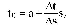
that hopefully converges to a root of f(t). The integral in the formula (14.26) is evaluated in [ShaT82] via Romberg integration that worked better than the trapezoidal or Simpson method. Furthermore, the fact that arc length is often roughly proportional to the parametric value motivated the authors to use the following starting value

where

This method for computing the arc-length parameterization seemed to work well for [ShaT82] and had no problems with convergence.

Sometimes one needs both arc lengths and arc-length parameterizations. In that case one can use the arc-length algorithm from [GueP90]. The tabledescribed earlier not only helps with arc length but also with arc length parameterization. If we want to find u so thatthen    we    find    the    j    so    that.    This will tell us thatand    give    us    a    much    better    starting    point    for    the    Newton-Raphson method applied to (14.26) so that it will run faster.

A problem related to finding the arc length of a curve is to find a curve between two points that has specified tangent lines at the endpoints and also has a specified length. See [RouB96a] and [RouB96b].