Cardiomyopathy Detection from Electrocardiogram Features (Classification, Evaluation and Management of Cardiomyopathies) Part 2

Oppositional BBO

Opposition-based learning (OBL) has been introduced as a method that can be used by Evolutionary Algorithms (EAs) to accelerate convergence speed by comparing the fitness of an individual to its opposite and retaining the fitter one in the population (Rahnamayan, Tizhoosh, & Salama, 2007; Tizhoosh, 2005). The "opposite" of an individual is defined as the reflection of that individual’s features across the midpoint of the search space. Opposition-based differential evolution (ODE) (Rahnamayan, Tizhoosh, & Salama, 2008.) was the first application of OBL to Evolutionary Algorithms (EAs). OBL was first incorporated in BBO in earlier research study (Ergezer, Simon, & Du, 2009) and was shown to improve BBO by a significant amount on standard optimization benchmarks.

Given an Evolutionary Algorithm (EA) population memberthere are at least three different types of oppositional points that can be defined. These oppositional points are referred to as the oppositethe quasi-oppositeand the quasi-reflected-opposite xr. Figure 3 illustrates these points for an arbitrary x in a one-dimensional domain. The point c is the center of the domain,the reflection of x acrossis a randomly generated point from a uniform distribution between c and■ is a randomly generated point from a uniform distribution between x and c.

Fig. 3. Illustration of an arbitrary EA individual x, its opposite x„, its quasi-opposite Xq, and its quasi-reflected-opposite xr, in a one-dimensional domain.

OBL is essentially a more intelligent way of implementing exploration instead of generating random mutations. Another way of viewing OBL is from the perspective of social revolutions in human society. Society often progresses on the basis of a few individuals who embrace philosophies that are not just random, but that are deliberately contrary to accepted norms. Given that an EA individual is described by the vector x, and that the solution to the optimization problem is uniformly distributed in the search domain, it is shown in Rahnamayan’ study (Rahnamayan, Tizhoosh, Salama, 2007) that xq is probably closer to the solution than x or x0. Further, it is presented in our earlier publication (Ergezer, Simon, & Du, 2009) that xr is probably closer to the solution than x9. These results are nonintuitive, but results related to random numbers are often nonintuitive, and the OBL results are derived not only analytically by also using simulation.

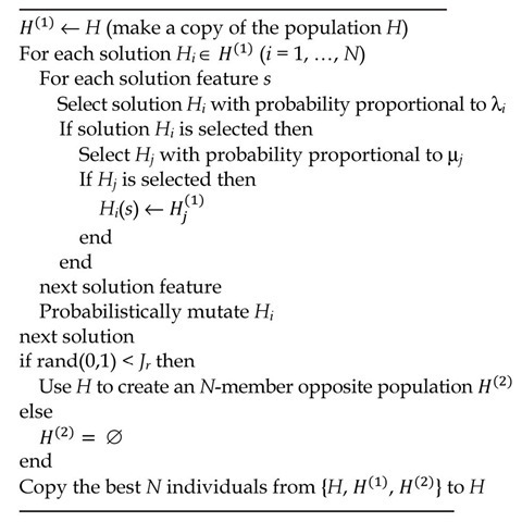
In this paper we use oppositional BBO (OBBO) to train the neuro-fuzzy ECG classification network. Suppose that the population size is N. OBBO works by generating a population of N opposite individuals which are the opposite of the current population. Then, given the entire 2N individuals comprised of both the original and the opposite populations, the best N individuals are retained for the next population. However, this does not occur at each generation. Instead it occurs randomly with a probability of Jr at each generation. Jr is called the jump rate. Based on (Rahnamayan, Tizhoosh, & Salama, 2006) we use Jr = 0.3 in this paper. In order to increase the likelihood of improvement at each generation we implement OBBO as follows. At each generation, we save the original population of N individuals before creating a population of N new individuals via migration. We then create an opposite population of N additional individuals if indicated by the jump rate. Of the total 2N or 3N individuals, we finally select the best N for the next generation. Note that this approach guarantees that the best individual in each generation is at least as good as that of the previous generation. This is similar to aevolutionary strategy (Du, Simon, & Ergezer, 2009), whose parameters are not to be confused with themigration parameters in BBO. The resulting OBBO algorithm is summarized in Figure 4.

Fig. 4. One generation of oppositional BBO (OBBO).

ECG data

In preparation for the testing of a cardiomyopathy diagnosis model, a database of long-duration ECG signals was collected. The database includes signals from 55 subjects, 18 of them with cardiomyopathy. Not all subjects experienced chronic or paroxysmal atrial fibrillation. The cardiomyopathy group contained 10 males and 8 females with a mean age of 54 (range 23-88) years. The control group contained 22 males and 15 females with a mean age of 60 (range 27-77) yrs. The inclusion criteria were the same for both groups: no chronic or paroxystic atrial fibrillation and no perioperative pacing.

ECG parameters describing P wave morphology were computed for each minute of data recording for all 55 patients in the training data set. This set of ECG parameter values constitutes the input component of the training data set for neuro-fuzzy model development. For additional details of ECG parameter computation algorithms see (Bashour et al., 2004; Visinescu et al., 2004; Visinescu, 2005; Visinescu et al., 2006; Ovreiu et al., 2008)

The P wave from the electrocardiogram reflects the electrical activity of the atria and may indicate the existence of irregularities in electrical conduction. Using a previously developed P wave detection method, the starting, ending, and maximum points of the P wave were determined (Visinescu, 2005). The average P wave morphology parameters were computed once per minute. The P wave morphology parameters included the following:

a. Duration

b. Amplitude

c. A shape parameter which represents monophasicity or biphasicity

d. Inflection point, which is the duration of the P wave between the onset and the peak points

e. Energy ratio, defined as the fraction between the right atrial excitation energy and the total atrial excitation energy.

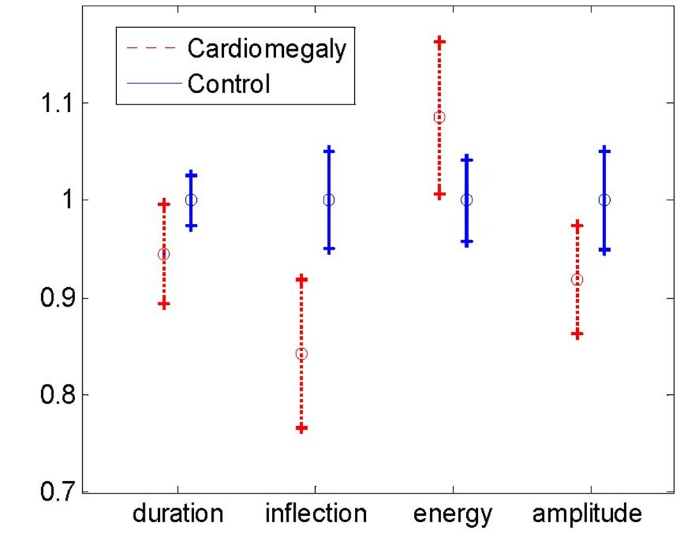
Initial investigation revealed that the monophasicity / biphasicity parameter did not vary appreciably between cardiomyopathy and control patients. We therefore discarded the monophasicity / biphasicity parameter from our data set. Differences between the remaining P wave morphology parameters for cardiomyopathy and control patients in the training database are presented in Figure 5. Based on the standard deviation bars, there is apparently important information included in these parameters. Their usefulness in identifying the patients with cardiomyopathy is determined by the proposed neuro-fuzzy model as discussed in the following section.

Fig. 5. P wave characteristics of cardiomyopathy and control patients. Data are normalized to the mean values of the control patients. Error bars show one standard deviation.

Experimental results

Problem setup

Cardiomyopathy diagnosis is performed by a multivariate, neuro-fuzzy classification model that uses current values of ECG P wave parameters to generate a cardiomyopathy classification index. The initial model is a multi-input single-output fuzzy inference system with a three-layer architecture (Figure 1). The fuzzification layer takes crisp parameter values and determines their memberships in linguistic categories (low, medium, high, etc.).

Each of these fuzzy variables are then input to each node of the fuzzy rule layer (i.e., the middle layer shown in Figure 1). The model output, which is the cardiomyopathy classification index, is the weighted average of the output rules.

Since we have four inputs (see Figure 5), we have m = 4 in Figure 1. The number of middle-layer neurons is equal to p and should be chosen as a tradeoff between good training performance and good generalization. If p is too small then training performance will be poor because we will not have enough degrees of freedom in the neuro-fuzzy network. If p is too large then test performance will be poor because the training algorithm will tend to "memorize" the training inputs rather than obtaining a good generalization for test data. The output y shown in Eq. (4) is chosen to be +1 for cardiomyopathy patients and -1 for control patients. The ECG database is used for training and the output of the neuro-fuzzy system is compared to the known classification of the ECG patient. The RMS training error is defined as

where N is the number of training inputs, di is the desired output of the ith training datum is the corresponding neuro-fuzzy output. In order to determine the best value of p (the number of middle-layer neurons) we run 10 Monte Carlo simulations with various values for p and compare training and testing errors. The BBO parameters that we use are as follows:

• Population size = 200

• Mutation rate = 2% per solution feature

• Generation limit = 50

Mutation is implemented by randomly generating a new parameter from a uniform distribution between the minimum and maximum parameter bounds. The parameter bounds that we use are as follows:

• Output singletons

• Membership centroids

• Membership standard deviations

We use ECG data from 55 test subjects as described in Section 3, which includes 37 control patients and 18 cardiomyopathy patients. We randomly divide the patients into approximately equal numbers of training patients and test patients. We therefore have 9 cardiomyopathy patients and 19 control patients for training the network, and 9 cardiomyopathy patients and 18 control patients for testing the network. We randomly choose 200 ECG data points from a 700-minute time interval for each patient for both training and testing. Therefore, we have 200x(9+19) = 5600 data points for training, and 200x (9+18) = 5400 data points for testing.

Parameter tuning and results

Table 1 shows the minimum training error attained as specified in Eq. (2) for various numbers of middle-layer neurons, along with the resulting correct classification rate for training and testing. An ECG data point is classified as cardiomyopathy if the neuro-fuzzy outputand control if the neuro-fuzzy outputThe quantity of primary interest is the correct classification rate for the test data, and Table 1 shows that this is attained with 3 middle-layer neurons. Fewer neurons gives too few degrees of freedom, and more neurons results in a tendency of the neuro-fuzzy system to overfit the training data and hence not provide adequate generalization for the test data.

p	Training Error		Train CCR (%)		Test CCR (%)
	Best	Mean	Best	Mean	Best	Mean
2	0.85	0.88	76	72	66	58
3	0.77	0.84	82	77	75	62
4	0.78	0.83	84	77	65	55
5	0.78	0.83	82	76	63	58

Table 1. Training error and correct classification rate (CCR) for training and testing as a function of the number of middle layer neurons p.

Next we implement OBBO to explore the effect of OBL on classification performance. Table 2 shows results for three different OBL options: standard BBO, OBBO using quasi-opposition (Q-BBO), and OBBO using quasi-reflected opposition (R-BBO). We use the same population size, mutation rate, and generation limit as discussed earlier. We use 3 middle-layer neurons as indicated by Table 1. Table 2 shows that OBBO using quasi-opposition provides the best neuro-fuzzy classification performance when test performance is used as the criterion.

Note that the numbers in Tables 1 and 2 do not match exactly because they are the results of different sets of Monte Carlo simulations. In future work we will use a more extensive set of simulations in order to obtain results with a smaller margin of error.

	Training Error		Train CCR (%)		Test CCR (%)
	Best	Mean	Best	Mean	Best	Mean
BBO	0.77	0.86	84	76	66	58
Q-BBO	0.83	0.86	79	74	69	62
R-BBO	0.80	0.85	81	75	65	60

Table 2. Training error and correct classification rate (CCR) for training and testing for alternative implementations oppositional BBO.

After settling on Q-BBO with 3 middle-layer neurons, we explore the effect of mutation rate on Q-BBO performance. Table 3 shows neuro-fuzzy results for various mutation rates. We use the same population size and generation limit as before. Table 3 shows that mutation rate does not have a strong effect on neuro-fuzzy system results, but based on test data performance, a low mutation rate generally gives better results than a high mutation rate.

Mutation rate (%)	Training Error		Train CCR (%)		Test CCR (%)
	Best	Mean	Best	Mean	Best	Mean
0.1	0.79	0.85	81	76	71	61
0.2	0.82	0.86	80	75	72	59
0.5	0.77	0.85	82	76	69	62
1.0	0.80	0.85	80	74	67	57
2.0	0.83	0.86	79	74	69	62
5.0	0.82	0.87	81	74	68	58
10.0	0.80	0.87	78	73	65	59

Table 3. Training error and correct classification rate (CCR) for different mutation rates using Q-BBO.

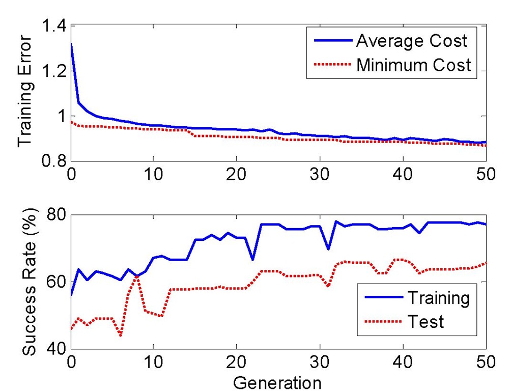
Figure 6 shows the progress for a typical Q-BBO training simulation. Note that the minimum training error in the top plot is monotonically nonincreasing due to the inherent elitism of the algorithm (see Figure 3). However, the average cost in the top plot, along with the success rates in the bottom plot, sometimes increases and sometimes decreases from one generation to the next. The results shown in Figure 6 also indicate that better results might be obtained if the generation limit were increased. However, care must be taken when increasing the generation limit. As the generation count increases, the training error will continue to decrease but the test error will eventually begin to increase due to overtraining (Tetko, Livingstone,& Luik, 1995).

The Q-BBO training run illustrated in Figure 6 resulted in the following neuro-fuzzy parameters:

Recall that we used a c range ofbut from Eq. (3) the highest membership centroid was less than 1 after Q-BBO training. This indicates that we could decrease the c range in order to get better resolution during training.

Similarly, recall that we used a ct range of [0.01, 5], but from Eq. (4) the highest standard deviation was less than 2 after Q-BBO training. This indicates that we could decrease the ct range in order to get better resolution during training.

Finally, recall that we used an output singleton z range of [-10, +10], but from Eq. (5) the output singletons were between -1 and 2 after Q-BBO training. This indicates that we could decrease the z range in order to get better resolution during training.

Fig. 6. Typical Q-BBO training results.