Image enhancement and restoration use similar operators but are driven by different goals. Image restoration is a process specifically designed to counteract known image degradation: for example, to improve the overall point-spread function of an image. Image enhancement is a user-driven process to meet specific image quality criteria: for example, noise reduction, sharpening, or edge enhancement. Operators for image enhancement and restoration are called filters. Two different types of filters exist: spatial-domain filters, which are generally based on convolution operations, and frequency-domain filters, which apply a defined frequency-response function. Frequency-domain filters are covered in more detail in Section 3.2; in this section we focus on convolution-based filters. The one-dimensional convolution of a function f (t) with another function, g(t), often referred to as the kernel, is defined as
where the symbol © indicates the convolution operation. The integral in Equation (2.7) needs to be evaluated for all possible values of t. It can be seen from the equation that f and g are shifted against each other for different values of t. The center of the function g is always where t = t , and the center of f is always where t = 0. The convolution operation becomes more intuitive in the discrete form, particularly when a kernel with finite support (-m to +m) is assumed:
Let us assume two kernel examples, with m = 1 in both cases. For kernel gi, the element at index -1 is 0.25, the element at index 0 is 0.5, and the element at index 1 is 0.25. Kernel g2 contains the elements -1,0, and 1 at index -1,0, and 1, respectively. With m = 1, the summation takes place for i = k – 1, k, and k + 1. In this special case, the convolution in Equation (2.8) becomes the summation
The first example, with kernel g1, is a moving-window weighted average; the kth element of the convolution result is computed from the weighted average of the kth element of the original time series and its two neighbors. The second example, with kernel g2, turns out to be a central-difference formulation that computes the first derivative except for a scaling factor.
In two dimensions, the convolution equation extends to
where I(x,y) is the original image convolved with a two-dimensional kernel g that has (2m + 1)2 elements. Depending on the kernel, convolution operations can be used, for example, to reduce noise, to sharpen the image, or to extract edges. Most often, the kernel g is quadratic and symmetric, so that the convolution becomes rotation-independent. The moving-average kernel, introduced in one dimension above [Equation (2.9)], can be extended to two dimensions and becomes
This kernel is a rough approximation of a Gaussian function with a standard deviation ct = 1.2, restricted to a 3 x 3 support and represented by integer elements. Note that the kernel is normalized so that the sum of its elements is unity. This normalization is necessary to conserve the amplitude of the image convolved with this kernel. Another consideration is the behavior of the convolution at the edges of the image. When a 3 x 3 kernel is used, the computation of the first and last image rows and columns requires that we access image values outside the image range (e.g., at x =-1 and y =-1). Since image data at these coordinates generally are not available, edge behavior needs to be defined. Four different methods are commonly used. In the first method, all values outside the image area can simply be assumed to be zero. This zero-padding method, although very simple to implement, has the disadvantage that it tends to create a discontinuity at the image edge. This discontinuity would negatively affect smoothing filters or edge detectors. Alternatively, a second method continues the closest edge value. Under this assumption, for example, I(x,y) = I(0,y) for all x < 0. This edge definition is frequently implemented, as it has minimal negative effects on convolution filters. The third alternative is a mirror definition; that is, in the example of the left boundary, I(x,y) = I(-x,y) for all x < 0. This boundary definition replicates the texture irregularity (e.g., frequency components, noise) of the pixels near the boundary. In most cases it behaves in a manner very similar to the second definition. A fourth definition "tiles" the image, that is, I(x,y) = I(x + N, y) for all -N < x < 0, where N is the number of pixels in the x-direction. This edge definition is not commonly used except in some cases where the periodicity assumption that underlies the Fourier transform plays an important role. The main disadvantage of the fourth definition is the possible occurrence of discontinuities at the boundary, very much like the zero-padding method.
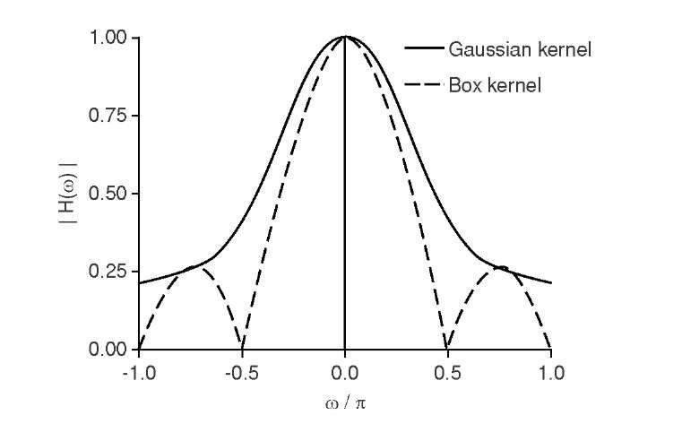
The kernel in Equation (2.11) is commonly used for weak noise reduction and moderate blurring, and the convolution with this kernel is often referred to as a smoothing operation. Stronger smoothing is possible with different kernel values to approximate Gaussian functions with larger standard deviations. When staying within the 3 x 3 confines of commonly used kernels, the extreme case would consist of a kernel with G(x,y) = 1 for all x,y inside the 3 x 3 support and a normalization factor of 9. Although this "box kernel" has a stronger smoothing action than the kernel in Equation (2.11), its frequency response shows undesirable characteristics. The convolution theorem (see Section 3.2) stipulates that a convolution of two functions corresponds to multiplication of the Fourier transforms of these functions. As can be seen in Figure 2.3, the box kernel with its abrupt transition from 1 to 0 has a steeper transition from the low frequencies H(m) = 1 (those that are allowed to pass, the passband) to higher frequencies (those that are stopped, the stopband).
FIGURE 2.3 Frequency responses of the Gaussian and the box smoothing kernel. While the box kernel shows a steeper drop-off near low spatial frequencies (m = 0), it completely suppresses certain frequencies and allows higher frequencies to pass again. The Gaussian kernel has less smoothing action, but it does not show undesirable behavior in the stopband.
However, after the box kernel reaches zero and fully suppresses the associated spatial frequency, even higher frequencies are allowed to pass again, albeit attenuated. The Gaussian kernel does not exhibit this behavior. The frequency response drops monotonically toward higher frequencies, although it drops off slower than the box kernel, and therefore its filtering action is weaker. To avoid the undesirable frequency response of the box kernel, yet provide a stronger filter with a steeper transition from the passband to the stopband, a larger kernel size is necessary to allow a smooth drop-off of the kernel values while allowing a large standard deviation. A suggested Gaussian approximation with a kernel size of 5 x 5 computed from a Gaussian function with a standard deviation of ct = 1.7 is
The smoothing action of a convolution with the kernel in Equation (2.12) is stronger than a convolution with the kernel in Equation (2.11). This conclusion can be reached by a different consideration. If the kernel in Equation (2.11) is applied twice, the linearity of the convolution operation allows the identity
The kernel in Equation (2.11) convolved with itself leads to a 5 x 5 kernel somewhat similar to the 5 x 5 kernel in Equation (2.12). Even larger smoothing kernels can be designed in the same manner. However, computational effort for the convolution increases with the square of the kernel size, specifically with N2m2, where the image is of size N x N and the kernel is of size m x m. Although the convolution can be implemented with fast integer operations, filtering in the frequency domain becomes more efficient when kernel sizes grow very large.
The operation complementary to smoothing is usually referred to as sharpening. A physical motivation for the design of a sharpening kernel was given by Russ,22 who suggested that blurring can be modeled as a diffusion process that follows the partial differential equation
where![]() is the Laplacian operator and k isthe diffusion constant. In its time-discrete form, Equation (2.14) becomes
is the Laplacian operator and k isthe diffusion constant. In its time-discrete form, Equation (2.14) becomes![]() . where t is the time step from iteration h to h + 1. An approximate reversal of the diffusion process in time would be
. where t is the time step from iteration h to h + 1. An approximate reversal of the diffusion process in time would be ![]() where the Laplacian of the blurred image gets subtracted from the image. The Laplacian operator, or second-derivative operator, can be discretized by finite differences. One-dimensional kernels of [-1 1 0]and[0 -1 1] realize discrete asymmetrical differences. The difference of the first-order differences becomes [1 -2 1]. In two dimensions, the Laplacian operator is often approximated by kernel L4 or L8:
where the Laplacian of the blurred image gets subtracted from the image. The Laplacian operator, or second-derivative operator, can be discretized by finite differences. One-dimensional kernels of [-1 1 0]and[0 -1 1] realize discrete asymmetrical differences. The difference of the first-order differences becomes [1 -2 1]. In two dimensions, the Laplacian operator is often approximated by kernel L4 or L8:
To enhance a blurred image, its convolution with the Laplacian kernel gets subtracted from the image (I’ = I – kI © L8), and because of the linearity of the convolution, the operation can be combined into a single convolution with the sharpening kernel S defined for k = 1:
In some software packages (NIH Image and ImageJ), the convolution with S in Equation (2.16) is termed "sharpen more," and the regular sharpening operation uses a kernel with weaker action where k = 0.25:
A convolution with a sharpening kernel has a highpass character; that is, high spatial frequencies get amplified. Small image detail and edges contain high-frequency components. Therefore, edges become more prominent after a sharpening operation. In addition, noise gets amplified.
Two more convolution-based filters with a highpass character are unsharp masking and DoG operators. Unsharp masking is an operation to remove inhomogeneous background from the image. The image is convolved with a very large Gaussian kernel so that ideally all detail information is removed by blurring. The blurred image is then subtracted form the original image. The difference-of-Gaussian (DoG) operator is closely related to the Laplacian operator. Again, larger kernel sizes are used. The DoG kernel is a Gaussian function with lower peak value and larger standard deviation subtracted from another Gaussian function that has a smaller standard deviation and a larger peak value.
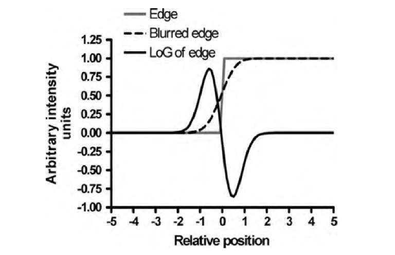
The noise-amplifying property of highpass filters is even more pronounced with the Laplacian kernel L in Equation (2.15). For this reason, a convolution with L rarely yields satisfactory results. However, Gaussian smoothing (for noise reduction) and computation of the second derivative with the Laplacian operator can be combined into a commonly used edge detection method, the Laplacian-of-Gaussian (or LoG) operator. An image first gets convolved with a large Gaussian kernel, and the result is convolved with the Laplacian. With the linearity of the convolution operation, the Gaussian and Laplacian kernels can be joined into a precomputed LoG kernel. Because a strong smoothing action is desired, LoG kernels are usually large. The principle of the LoG-based edge detector is demonstrated in Figure 2.4. It is fundamental to have strong blurring to create a soft transition instead of a sharp edge. This does not only suppress noise. The second derivative of the blurred edge crosses through zero at the location of the edge, and a wider (less steep) transition allows for easier detection of the zero-valued edge points.
FIGURE 2.4 Edge detection with the Laplacian-of-Gaussian (LoG) operator. A discontinuity (edge) is blurred by a convolution with a Gaussian kernel. The second derivative of the blurred edge crosses through zero exactly at the position of the edge.
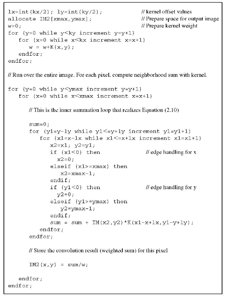
Algorithm 2.3 Convolution of an image IM(x,y) with a kernel K(x,y). The image size is xmax and ymax. The kernel size is kx and ky, both of which need to be odd-valued integers. A convolution cannot be performed in-place. Therefore, the result is stored in IM2(x,y). At the image edges, the image is assumed to continue its edge value indefinitely. The kernel does not need to be normalized; this is handled with the variable w. The kernel K(x,y) needs to be filled with values in advance: for example, from Equation (2.11) or (2.15).
An example of how a convolution of an image with an arbitrary kernel can be implemented is shown in Algorithm 2.3.


