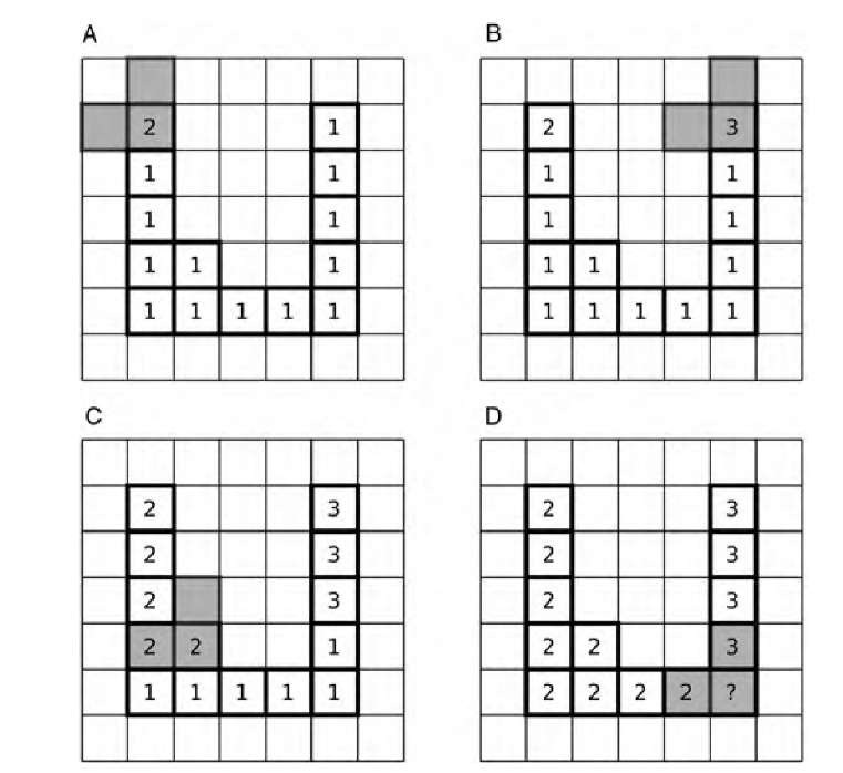
Most image processing software contain functions to distinguish different features in an image. These are often referred to as feature labeling, particle analysis, or cluster analysis. The most widely applied and most efficient approach to label image features is a two-pass process. The input image to this process is assumed to be strictly binary, with the value 1 representing feature pixels and the value 0 representing background pixels. A counter exists that starts at a value of 2. In the first pass, the image is scanned from left to right and from top to bottom: If a nonzero pixel has a nonzero neighbor to the left or above, it assumes the value of that neighbor; if the scan runs across a nonzero pixel with background pixels to the left and above, it assumes the value of the counter, and the counter is incremented. After the first pass finishes, all features are now assigned different image values. However, some features may contain more than one value (e.g., in U-shaped features). For this reason, a second pass is required in which features that contain connected regions with different image values are renumbered until each feature contains only pixels with one unique value. The process of cluster labeling is illustrated in Figure 9.3. The example is a U-shaped feature, and at the end of the first pass, connected subclusters with more than one value exist. These cases where one feature contains ambiguous numbering need to be resolved in a separate pass.
An alternative and potentially slightly less efficient algorithm can be devised that labels the clusters in one pass. This algorithm scans the binary input image from left to right and from top to bottom, similarly with a counter that starts at a value of 2. Each time the scan encounters a pixel with the value of 1, a region-growing process is initiated, and the fully grown region is filled with the value of the counter. The counter is then incremented. The advantage of the second algorithm lies in its more straightforward implementation. The process of feature labeling and the extraction of three sample shape descriptors (aspect ratio, compactness, and irregularity, as defined in Section 9.2) for each feature is outlined in Algorithms 9.1 and 9.2. Algorithm 9.2 builds on Algorithm 9.1. The input image needs to be thresholded and is assumed to be strictly binary; that is, all background pixels have a pixel value of zero and all feature pixels have a value of 1. Algorithm 9.2 detects unlabeled features, whereas Algorithm 9.1 does the actual labeling of an individual feature by region growing and the determination of its shape descriptors. In the process of region growing, each feature’s centroid and boundary can be computed. The centroid is the average of all feature pixel coordinates, and a boundary pixel is any pixel that touches a background pixel. At the end of Algorithm 9.2, the tables for irregularity, compactness, aspect ratio, and size can be used as lookup tables, or to relabel the clusters according to their features. This algorithm was used to generate Figure 9.1C.
FIGURE 9.3 Cluster labeling with the two-pass method. The image is scanned from left to right and from top to bottom with an inverted-L shape (pixels marked gray). If the corner pixel of the inverted L reaches a new feature (indicated by the value 1), the algorithm begins a new cluster and assigns to it a cluster number greater than 1 (A). The algorithm cannot see that the pixel that was discovered in part B belongs to the same cluster, and both subgroups of connected pixels are treated as separate clusters (C). This leads to an ambiguity in part D. The ambiguity can be resolved by assigning one of the two possible values and merging connecting subclusters in a separate pass.

