INTRODUCTION
Proposed in 1962, the Hough transform (HT) has been widely applied and investigated for detecting curves, shapes, and motions in the fields of image processing and computer vision. However, the HT has several shortcomings, including high computational cost, low detection accuracy, vulnerability to noise, and possibility of missing objects. Many efforts target at solving some of the problems for decades, while the key idea remains more or less the same. Proposed in 1989 and further developed thereafter, the Randomized Hough Transform (RHT) manages to considerably overcome these shortcomings via innovations on the fundamental mechanisms, with random sampling in place of pixel scanning, converging mapping in place of diverging mapping, and dynamic storage in place of accumulation array. This article will provides an overview on advances and applications of RHT in the past one and half decades.
BACKGROUND
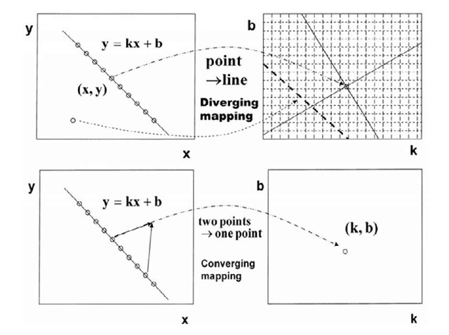
Taking straight line detection as an example, the upper part of Fig. 1 shows the key idea ofthe Hough Transform (HT) (Hough, 1962) . A set of points on a line y=kx+b in the image are mapped into a set of lines across a point (k, b) in the parameter space. A uniform grid is located on a window in the (k, b) space, with an accumulator a(k, b) at each bin. As each point (x,y) on the image is mapped into a line in the (k, b) space, every associated accumulator a(k, b) is incremented by 1. We can detect lines by finding every accumulator with it’s score a(k, b) larger than a given threshold.
Figure 1. From hough transform to randomized hough transform
The Hough Transform was brought to the attention of the mainstream image processing community by Rosenfeld (1969). Then Duda and Hart (1972) not only introduced the polar parameterization technique for more efficient line detection, but also demonstrated how a circle can be detected. Kimme, Ballard and Sklansky (1975) made circular curve detection significantly more effective by using the gradient information of pixels. Merlin and Faber (1975) showed how the HT could be generalized to detect an arbitrary shape at a given orientation and a given scale. Ballard (1981) eventually generalized the HT to detect curves of a given arbitrary shape for any orientation and any scale. Since then, a lot of applications, variants and extensions of the HT have been published in the literature. A survey on these developments of the HT is given by Illingworth and Kittler (1988).
However, the HT has several critical drawbacks as follows:
a. All pixels are mapped, and every bin in the grid needs an accumulator. If there are d parameters, each represented by M bins or grid points, one needs M accumulators.
b. To reduce the computational cost, quantization resolution cannot be high, which blurs the peaks and leads to low detection accuracy.
c. Each pixel activates every accumulator located on a line, but there is only one that represents the correct one while all the others are disturbances.
d. If the grid window is set inappropriately, some objects may locate outside the window and thus cannot be detected.
e. Disturbing and noisy pixels cause many interfering accumulations.
Many efforts have been made to alleviate these problems. Using the gradient information of pixels is one of them. Another is analyzing noise and error sensitivity (vanVeen, 1981; Brown, 1983; Grimson & Huttenlocher, 1990). The third is the use of hierarchical voting accumulation (Li, Lavin & LeMaster, 1986) or multiresolution (Atiquzzaman, 1992). Yet another is improving the effect of quantization through the use of kernels (Palmer, Petrou, & Kittler, 1993) or error propagation analysis (Ji & Haralick, 2001), as well as hypothesis testing (Princen, Illingworth, & Kittler, 1994). However, none of these suggestions offer any fundamental changes to the key mechanisms of HT.
Proposed in 1989 and further investigated thereafter (Xu, Oja, & Kultanen, 1990; Xu & Oja, 1993), the Randomized Hough Transform (RHT) tackles the above problems by using a fundamental innovation: the one-to-many diverging mapping from the image space to the parameter (accumulator) space, as shown in the upper part of Fig.1(a), is replaced by a many-to-one converging mapping, as shown in the bottom part of Fig.1(a). This fundamental change further enables several joint improvements, such as a random sampling in place of pixel scanning, a small size dynamic storage in place of the array of Md accumulators, and an adaptive detection in place of enumerating all the pixels and picking those accumulators with scores larger than a threshold. As a result, not only time and storage complexity have been reduced significantly, but also the detection accuracy has been improved considerably.
Subsequently, many studies have been made on RHT. On one hand, there are various real applications such as medical images (Behrens, Rohr, & Siegfried, 2003), range images (Ding, et al, 2005), motion detection (Heikkonen, 1995), object tracking for a mobile robot (Jean & Wu, 2004), soccer robot (Claudia, Rous, & Kraiss, 2004), mine detection (Milisavljevic, 1999), and others (Chutatape & Guo, 1999). On the other hand, there are also many further developments on RHT, including an efficient parameterization for ellipse detection (McLaughlin, 1998), extension to motion detections (Kalviainen, Oja, & Xu, 1991; Xu, 2007), the uses of local gradient information, local connectivity and neighbor-orientation for further improvements (Brailovsky, 1999; Kalviainen & Hirvonen, 1997), an integration with error propagtion analysis (Ji & Xie, 2003), a modification of random sampling to importance sampling (Walsha & Raftery, 2002), and others (Xu, 2007). Due to space limit, it is not possible to provide a complete survey here. An early review on RHT variants is referred to (Kalviainen, Hirvonen, Xu, & Oja, 1995), and recent elaborations on RHT are referred to (Xu, 2007).
It may also need to be mentioned that the literature on RHT studies often includes studies under the name of probabilistic HT (Bergen & Shvaytser, 1991; Kiry-ati, Eldar & Bruckstein, 1991) that also suggests to use a random sampling to replace the scanning in the implementation of the standard HT and thus shares one of the previously mentioned RHT features. However, it will not lose too much generality to regard it as a degenerated case of RHT for an understanding purpose, though there are some detailed differences.
BASIC RHT MECHANISMS AND CHARACTERISTICS
As shown in Fig.1, one pixel is mapped into all the points on a line passing (k,b) by the diverging mapping mechanism of HT, which actually incurs the above drawbacks (a)-(e). RHT replaces this mechanism with a converging mapping mechanism such that two or more pixels are picked to jointly determine a line, i.e., mapped into one point (k,b). By this mechanism, different points on the same line y=kx+b will hit the same point (k,b), without creating a great number of false accumulations. Also, the feature of being mapped into one point at a time makes it possible to construct accumulators dynamically, with no need of laying a grid on a pre-specified window. We only need to accumulate a(k, b) at those locations activated by the converging mappings. Also, quantization resolution may vary for different locations, and each quantization bin can be replaced by a kernel. As a result, the drawbacks (b),(c),(d) no longer exist.
Without considering the quantization effect, if there is a line consisting of n pixels on an image, we get a peak with n counts in its accumulated scores. Assume that in its neighbour there is another peak of false line consisting of m < n pixels, then the ratio n/m describes a signal/noise ratio of a reliable detection by HT. In RHT, assuming that we exhaust all the possible pairs of pixels, the voting counts for the line will be n(n-1)/2 while the voting counts for the disturbing false line will be m(m-1)/2, i.e., the signal/noise ratio becomes mkm—k that is m—” times increased compared to HT. Thus, the above problem (e) can also be significantly improved.
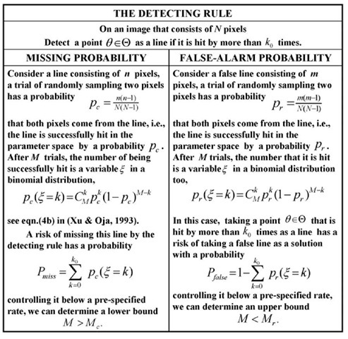
Table 1. Missing probability versus false alarm probability
In fact, it is not necessary to exhaust all the possible pairs of pixels for RHT to detect lines. Via randomly sampling two pixels for a converging mapping, we only need to have a small fraction of all the possible pairs to get the degree ^J) with a high probability, which solves the above problem (a) with a significant reduction in both time and space complexities. A more precise explanation is given in Tab.1. We detect a point 9e© as a line if it is hit by more than k0 times, with a risk of missing this line by a small probability Pmiss. Controlling it below a pre-specified rate, we need to only run M > Mc trails. On the other hand, controlling probability of taking a false line as a solution, we can determine an upper bound M< M. Even if a line is falsely detected, it can be later discarded by evaluating all the detected lines via the actual pixels on the image. Thus, a large will not affect the performance too much, but will only waste computing time.
RHT GENERAL FORM AND EXTENSIONS
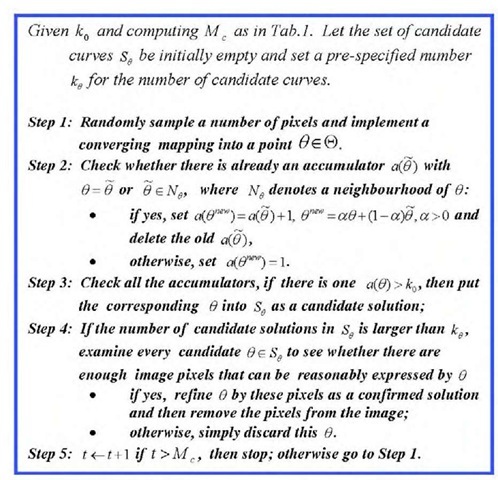
In general, RHT is applicable to a curve that can be expressed in a parametric equation f (x,y,9) = 0 with a number k of free parameters. Solving the j oint equations f (x,y,9) = 0, i = 1,…, k yields a converging mapping into a point 9e@. A general algorithmic form is given in Tab.2.
We can obtain variants and extensions by modifying either one or more of the first four steps in Tab.2. First, the converging mapping in Step 1 can be altered by varying either the way of getting samples, or the way of computing 9e© from these samples, or both. Instead of random sampling, samples can be obtained by searching a candidate solution in S9 via local connectivity and neighbor-orientation (Kalviainen, Hirvonen, Xu, & Oja, 1995; Brailovsky, 1999; Kalviainen & Hirvonen, 1997) or by importance sampling (Walsha & Raftery, 2002). Instead of solving joint equations, as discussed in (Xu, 2007), a solution can also be obtained by either a least square fitting, an Lpnorm fitting, or by maximum likelihood estimation. Sometimes, it may even consider under-constrained equations by taking less samples, from which a parametric curve or surface in © is obtained to implement an array based accumulation similar to HT.
Table 2. The general RHT in algorithmic form
Second, there are also alternatives for Step 2 and Step 3. One extreme is returning to an array based accumulation. The other extreme is that all the mapped points in © are stored as they are, and either cluster analysis or kernel based density estimation is made on them to find cluster centres and density degrees for detecting curves or objects. Between the two extremes, we may consider a trade off or their combination (Xu, 2007). Third, Step 4 can also be performed with different choices, including a S-band test, a fitting error threshold, and a hypothesis testing (Xu, 2007).
Moreover, instead of checking candidate solution every time t, we can let the procedure run until t = Mc, put those accumulators with a(9) > k0 into S0 as candidate solutions and examine these candidates at Step 4. Also, checking and examining candidates can be made per a pre-specified period. Furthermore, gradient information in a grey image may also improve the converging mapping.
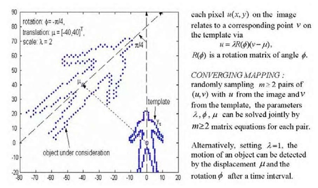
The last but not the least, RHT has also be extended to detect objects by a template as shown in Fig.2.
FUTURE TRENDS
Challenges to RHT mainly come from the effects of noise and quantization. Two types of noise are shown in Fig.3. The first type is in Fig.3(a) with disturbing pixels added but the original pixels unaffected. This noise type may reduce the signal/noise ratio, resulting in more computing time and space. However, the accuracy of the detected line will be not affected. The second type is in Fig.3(b), with some original pixels deviated from the exact line. The quantization effect can be regarded as a special case of this type that uniformly distributed noise is added to the coordinates of pixels. The second type not only reduces the signal/ noise ratio but also makes the detected line inaccurate. As yet, there lacks a systematic theoretical analysis on how the solution accuracy will be affected by this second type. More importantly, theoretical guides are lacking on how to control the accuracy of detected curves and objects.
The tasks of detecting curves and objects can also be performed from the perspective of mixture based learning, which is much more robust in the case of the second type of noise (Xu, 2003; Liu, Qiao, & Xu, 2006; Xu, 2007). Solving pattern recognition tasks by machine learning approaches is a popular trend in the past decade and currently. Actually, the machine learning perspective are complementary to the perspective of HT/RHT type evidence accumulation. A trend is integrating the strengths of both.
Figure 2. Use a template to match a shape via translation f, rotation ^ and scaling X
Figure 3. Different effects by two types of noises
CONCLUSION
This article provides not only a brief overview on nearly two decade developments and applications of RHT for detecting curves, shapes, and motions, but also a tutorial and re-elaboration on basic mechanisms, variants, and extensions of RHT, as well as challenges and future trends of RHT studies. Recently, a general problem solving paradigm has been developed and implemented by an integration of five essential mechanisms (Xu, 2007). Not only the difference between the machine learning perspective and HT/RHT perspective can be understood via handling two coupled core tasks, namely amalgamating evidences and discriminating differences, but also different implementations of these mechanisms and differences in a specific integration may bring us new results and potential directions for future studies.
KEY TERMS
S Band Test: A pixel is said to fall in the S band of p (it denotes a curve or surface ) in the image space if the shortest distance from this pixel to p is less than a pre-specified threshold S. Pixels falling in the S band of p are regarded as belonging to p, and a S band test can be designed according to these pixels.
Cluster Analysis: Beyond using an accumulation array, in the cases of a converging mapping, every mapped point in R is memorized. After an enough number of converging mappings, we get a set of points on which cluster analyses can be made to find clusters’ centre (mean or median).
Diverging Mapping vs. Converging Mapping: Given pixels of a number m, a set of under-constrained equations specify a curve or manifold of a dimension > k – m in R if m < k. E.g., from a line y=kx+b passing a given pixel in the image, we have a line b=y-kx in R. This case is called diverging mapping because m pixels are mapped diversely to the R space. On the other hand, if m > k, a unique point in the R space maybe determined by solving a set of joint equations or optimizing a cost when the joint equations are over-constrained, i.e., we have a converging mapping that maps m pixels into one point in R.
Kernel Estimator: Every mapped point is memorized as the centre of a kernel function, e.g., a bell-shaped such as a Gaussian. Collectively, mapped points forms a density estimation for a multi-mode distribution, with each mode in place of the above cluster centre.
Random Sampling: Given a set of Npixels, we take a number m of pixels with each picked randomly with a probability 1/N. Repeating this sampling by an enough number of times, a global configuration of Npixels will emerge, without enumerating all the N pixels.
Threshold Based Voting vs. Local Maxima Finding: Given a pre-specified threshold, an accumulator in an array is picked if it receives votes larger than the threshold, without considering any neighborhood. Finding a local maximum means to find an accumulator with its votes larger than those of accumulators located in its neighborhood area.
Under-Constrained vs. Over-Constrained Equations: For a parametric equation of k free parameters, we have a set of under-constrained equations with pixels of a number m < k and a set of over-constrained equations with pixels of a number m > k in a non-degenerate way.


