INTRODUCTION
Artificial neural networks (ANNs) (McCulloch & Pitts, 1943) (Haykin, 1999) were developed as models of their biological counterparts aiming to emulate the real neural systems and mimic the structural organization and function of the human brain. Their applications were based on the ability of self-designing to solve a problem by learning the solution from data. A comparative study of neural implementations running principal component analysis (PCA) and independent component analysis (ICA) was carried out. Artificially generated data ad-ditively corrupted with white noise in order to enforce randomness were employed to critically evaluate and assess the reliability of data projections. Analysis in both time and frequency domains showed the superiority of the estimated independent components (ICs) relative to principal components (PCs) in faithful retrieval of the genuine (latent) source signals.
Neural computation belongs to information processing dealing with adaptive, parallel, and distributed (localized) signal processing. In data analysis, a common task consists in finding an adequate subspace of multivariate data for subsequent processing and interpretation. Linear transforms are frequently employed in data model selection due to their computational and conceptual simplicity. Some common linear transforms are PCA, factor analysis (FA), projection pursuit (PP), and, more recently, ICA (Comon, 1994). The latter emerged as an extension of nonlinear PCA (Hotelling, 1993) and developed in the context of blind source separation (BSS) (Cardoso, 1998) in signal and array processing. ICA is also related to recent theories of the visual brain (Barlow, 1991), which assume that consecutive processing steps lead to a progressive reduction in the redundancy of representation (Olshausen and Field, 1996).
This contribution is an overview of the PCA and ICA neuromorphic architectures and their associated algorithmic implementations increasingly used as exploratory techniques. The discussion is conducted on artificially generated sub- and super-Gaussian source signals.
BACKGROUND
In neural computation, transforming methods amount to unsupervised learning, since the representation is only learned from data without any external control. Irrespective of the nature of learning, the neural adaptation may be formally conceived as an optimization problem: an objective function describes the task to be performed by the network and a numerical optimization procedure allows adapting network parameters (e.g., connection weights, biases, internal parameters). This process amounts to search or nonlinear programming in a quite large parameter space. However, any prior knowledge available on the solution might be efficiently exploited to narrow the search space. In supervised learning, the additional knowledge is incorporated in the net architecture or learning rules (Gold, 1996). A less extensive research was focused on unsupervised learning. In this respect, the mathematical methods usually employed are drawn from classical constrained multivariate nonlinear optimization and rely on the Lagrange multipliers method, the penalty or barrier techniques, and the classical numerical algebra techniques, such as deflation/renormalization (Fiori, 2000), the Gram-Schmidt orthogonalization procedure, or the projection over the orthogonal group (Yang, 1995).
PCA and ICA Models
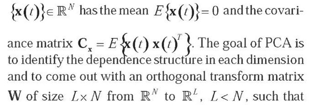
Mathematically, the linear stationary PCA and ICA models can be defined on the basis of a common data model. Suppose that some stochastic processes are represented by three random (column) vectors x(t), n(t)e RN and s (t)e RM with zero mean and finite covariance, with the components of s(t)= {s1 (t), s2 (t),…, sM (t)} being statistically independent and at most one Gaussian. Let A be a rectangular constant full column rank Nx M matrix with at least as many rows as columns (N> M), and denote by tthe sample index (i.e., time or sample point) taking the discrete values t = 1, 2, …,
T We postulate the existence of a linear relationship among these variables like:
Here s (t), x(t), n(t), and A are the sources, the observed data, the (unknown) noise in data, and the (unknown) mixing matrix, respectively, whereas at, i = 1,2,…,M are the columns of A. Mixing is supposed to be instantaneous, so there is no time delay between a (latent) source variable st (t) mixing into an observable (data) variable x.(t), with i = 1, 2, …, M and j = 1, 2, …, N.
Consider that the stochastic vector process
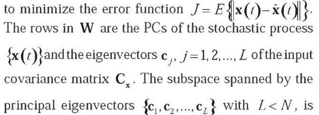
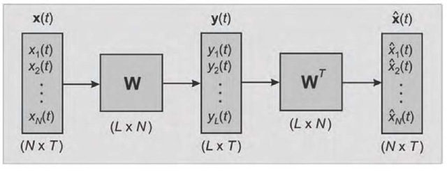
the L-dimensional output vector y (t)= W x (t) sufficiently represents the intrinsic features of the input data, and where the covariance matrix Cy of {y (t)} is a diagonal matrix D with the diagonal elements arranged in descending order, du > di+1i+1. The restoration
called the PCA subspace or dimensionality L.
The ICA problem can be formulated as following:
given T realizations of x (t), estimate both the matrix
A and the corresponding realizations of s (t). In BSS the task is somewhat relaxed to finding the waveforms
{ (0} of the sources knowing only the (observed)
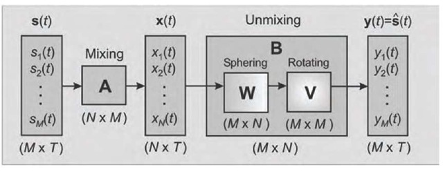
mixtures {xj (t)|. If no suppositions are made about the noise, the additive noise term is omitted in (1). A practical strategy is to include noise in the signals as supplementary term(s): hence the ICA model (Fig. 2) becomes:
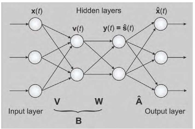
The source separation consists in updating an unmixing matrix B (t), without resorting to any information about the spatial mixing matrix A, so that the output vector y (t) = B (t) x (t) becomes an estimate y (t) = s (t) of the original independent source signals s (t). The separating matrix B (t) is divided in two parts dealing with dependencies in the first two moments, i.e., the whitening matrix V (t), and the dependencies in higher-order statistics, i.e., the orthogonal separating matrix W (t) in the whitened space (Fig. 2). If we assume zero-mean observed data x (t), then we get by whitening a vector v (t) = V (t) x (t) with decorrelated components. The subsequent linear transform W (t) seeks the solution by an adequate rotation in the space of component densities and yields y (t) = W (t) v (t) (Fig. 2). The total separation matrix between the input and the output layer turns to be B (t) = W (t) V (t) . In the standard stationary case, the whitening and the orthogonal separating matrices converge to some constant values after a finite number of iterations during learning, that is, B (t) ^ B = W V.
Figure 1. Schematic of the PCA model
Figure 2. Schematic of the ICA model
Figure 3. A simple feed-forward ANN performing PCA and ICA
NEURAL IMPLEMENTATIONS
A neural approach to BSS entails a network that has mixtures of the source signals as input and produces approximations of the source signals as output (Figure 3). As a prerequisite, the input signals must be mutually uncorrelated, a requirement usually fulfilled by PCA. The output signals must nevertheless be mutually independent, which leads in a natural way from PCA to ICA. The higher order statistics required by source separation can be incorporated into computations either explicitly or by using suitable nonlinearities. ANNs better fit the latter approach (Karhunen, 1996).
The core of the large class of neural adaptive algorithms consists in a learning rule and its associated optimization criterion (objective function). These two items differentiate the algorithms, which are actually families of algorithms parameterized by the nonlinear function used. An update rule is specified by the iterative incremental change AW of the rotation matrix W, which gives the general form of the learning rule:
Neural PCA
First, consider a single artificial neuron receiving an M-dimensional input vector x. It gradually adapts its weight vector w so that the function E {f (wTx is maximized, where E is the expectation with respect to the (unknown) probability density of x and f is a continuous objective function. The function /is bounded by setting constant the Euclidian norm of w. A constrained gradient ascent learning rule based on a sequence of sample functions for relatively small learning rates a (t) is then (Oja, 1995):
where g = f’. Any PCA learning rules tend to find that direction in the input space along which the data has maximal variance. If all directions in the input space have equal variance, the one-unit case with a suitable nonlinearity is approximately minimizing the kurtosis of the neuron input. It means that the weight vector of the unit will be determined by the direction in the input space on which the proj ection of the input data is mostly clustered and deviates significantly from normality. This task is essentially the goal in the PP technique.
In the case of single layer ANNs consisting of L parallel units, with each unit i having the same M-element input vector x and its own weight vector wy that together comprise an M x L weight matrix W = [w1,w 2,... ,w L ] the following training rule obtained from (4) is a generalization of the linear PCA learning rule (in matrix form):
Due to the instability of the above nonlinear Heb-bian learning rule for the multi-unit case, a different approach based on optimizing two criteria simultaneously was introduced (Oja, 1982):
Here (t) is chosen positive or negative depending on our interest in maximizing or minimizing, respectively, the objective function J (wy )= E {f (xTw t )} . Similarly, y (t) is another gain parameter that is always positive and constrains the weight vectors to orthonormality, which is imposed by an appropriate penalty function such as:
This is the bigradient algorithm, which is iterated until the weight vectors have converged with the desired accuracy. This algorithm can use normalized Hebbian or anti-Hebbian learning in a unified formula. Starting from one-unit rule, the multi-unit bigradient algorithm can simultaneously extract several robust counterparts of the principal or minor eigenvectors of the data co-variance matrix (Wang, 1996).
In the case of multilayered ANNs, the transfer functions of the hidden nodes can be expressed by radial basis functions (RBF), whose parameters could be learnt by a two-stage gradient descent strategy. A new growing RBF-node insertion strategy with different RBF is used in order to improve the net performances. The learning strategy is reported to save computational time and memory space in approximation of continuous and discontinuous mappings (Esposito et al., 2000).
Neural ICA
Various forms of unsupervised learning have been implemented in ANNs beyond standard PCA like nonlinear PCA and ICA. Data whitening can be neurally emulated by PCA with a simple iterative algorithm that updates the sphering matrix V (t):
After getting the decorrelation matrix V (t), the basic task for ICA algorithms remains to come out with an orthogonal matrix W (t), which is equivalent to a suitable rotation of the decorrelated data v (t )= V (t )x (t) aiming to maximize the product of the marginal densities of its components. There are various neural approaches to estimate the rotation matrix W (t) .An important class of algorithms is based on maximization of network entropy (Bell, 1995). The BS nonlinear information maximization (infomax) algorithm performs online stochastic gradient ascent in mutual information (MI) between outputs and inputs of a network. By minimizing the MI between outputs, the network factorizes the inputs into independent components. Considering a network with the input vector x (t), a weight matrix W (t), and a monotonically transformed output vector y = g (Wx + w 0), then the resulting learning rule for the weights and bias-weights, respectively, are:
In the case of bounded variables, the interplay between the anti-Hebbian term x (1 – 2y)T and the antidecay term [WT ]- produces an output density that is close to the flat constant distribution, which corresponds to the maximum entropy distribution. Amari, Cichocki, and Yang (Amari, 1996) altered the BS in-fomax algorithm by using the natural gradient instead of the stochastic gradient to reduce the complexity of neural computations and significantly improving the speed of convergence. The update rule proposed for the separating matrix is:
Lee et al. (Lee, 2000) extended to both sub-and super-Gaussian distributions the learning rule developed from the infomax principle satisfying a general stability criterion and preserving the simple initial architecture of the network. Applying either natural or relative gradient (Cardoso, 1996) for optimization, their learning rule yields results that compete with fixed-point batch computations.
The equivariant adaptive separation via independence (EASI) algorithm introduced by Cardoso and Laheld (1996) is a nonlinear decorrelation method. The objective function J(W)= E{f(Wx)} is subject to minimization with the orthogonal constraint imposed on W and the nonlinearity g = f’ chosen according to data kurtosis. Its basic update rule equates to:
Fixed-point (FP) algorithms are searching the ICA solution by minimizing mutual information (MI) among the estimated components (Hyvarinen, 1997). The FastICA learning rule finds a direction w so that the projection of wTx maximizes a contrast function
standing for the standardized Gaussian variable. The learning rule is basically a Gram-Schmidt-like decor-relation method.
ALGORITHM ASSESSMENT
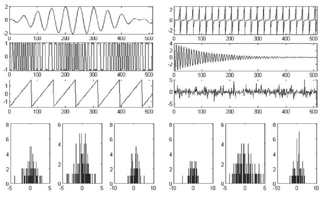
We comparatively run both PCA and ICA neural algorithms using synthetically generated time series additively corrupted with some white noise to alleviate strict determinism (Table 1 and Fig. 4.). Neural PCA was implemented using the bigradient algorithm since it works for both minimization and maximization of the criterion J1 under the normality constraints enforced by the penalty function J2.
The neural ICA algorithms were the extended infomax ofBell and Sejnowski, a semi-adaptive fixed-point fast ICA algorithm (Hyvarinen & Oja, 1997), an adapted variant of EASI algorithm optimized for real data, and the extended generalized lambda distribution (EGLD) maximum likelihood-based algorithm.
Table 1. The analytical form of the signals sources
Figure 4. Sub-Gaussian (left) and super-Gaussian (right) source signals and their corresponding histograms (bottom)
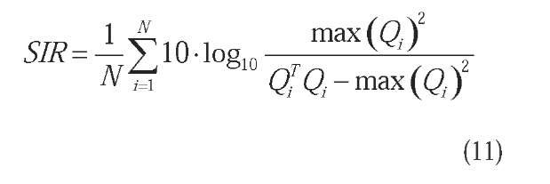
In the case of artificially generated sources, the accuracy of separating the latent sources by an algorithm performing ICA can be measured by means of some quantitative indexes. The first we used was defined as the signal-to-interference ratio (SIR):
where Q = BA is the overall transforming matrix of the latent source components, Q. is the i-th column of Q, max (Q) is the maximum element of Q, and N is the number of the source signals. The higher the SIR is, the better the separation performance of the algorithm.
A secondly employed index was the distance between the overall transforming matrix Q and an ideal permutation matrix, which is interpreted as the cross-talking error (CTE):
Above, Q.j is the j-th element of Q, max| Q.| is the maximum absolute valued element of the row i in Q, and max| Qj| is the maximum absolute valued element of the column j in Q. A permutation matrix is defined so that on each of its rows and columns, only one of the elements equals to unity while all the other elements are zero. It means that the CTE attains its minimum value zero for an exact permutation matrix (i.e., perfect decomposition) and goes positively higher the more Q deviates from a permutation matrix (i.e., decomposition of lower accuracy).
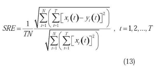
We defined the relative signal retrieval error (SRE) as the Euclidian distance between the source signals and their best matching estimated components normalized to the number of source signals, times the number of time samples, and times the module of the source signals:
The lower the SRE is, the better the estimates approximate the latent source signals.
The stabilized version of FastICA algorithm is attractive by its fast and reliable convergence, and by the lack of parameters to be tuned. The natural gradient incorporated in the BS extended infomax performs better than the original gradient ascent and is computationally less demanding. Though the BS algorithm is theoretically optimal in the sense of dealing with mutual information as objective function, like all neural unsupervised algorithms, its performance heavily depends on the learning rates and its convergence is rather slow. The EGLD algorithm separates skewed distributions, even for zero kurtosis. In terms of computational time, the BS extended infomax algorithm was the fastest, FastICA more faithfully retrieved the sources among all algorithms under test, while the EASI algorithm came out with a full transform matrix Q that is the closest to unity.
FUTURE TRENDS
Neuromorphic methods in exploratory analysis and data mining are rapidly emerging applications of unsu-pervised neural training. In recent years, new learning algorithms have been proposed, yet their theoretical properties, range of optimal applicability, and comparative assessment have remained largely unexplored. No convergence theorems are associated with the training algorithms in use. Moreover, algorithm convergence heavily depends on the proper choice of the learning rate(s) and, even when convergence is accomplished, the neural algorithms are relatively slow compared with batch-type computations. Nonlinear and nonstationary neural ICA is expected to be developed due to ANNs nonalgorithmic processing and their ability to learn nonanalytical relationships if adequately trained.
CONCLUSION
Both PCA and ICA share some common features like aiming at building generative models that are likely to have produced the observed data and performing information preservation and redundancy reduction. In a neuromorphic approach, the model parameters are treated as network weights that are changed during the learning process. The main difficulty in function approximation stems from choosing the network parameters that have to be fixed a priori, and those that must be learnt by means of an adequate training rule.
PCA and ICA have major applications in data mining and exploratory data analysis, such as signal characterization, optimal feature extraction, and data compression, as well as the basis of subspace classifiers in pattern recognition. ICA is much better suited than PCA to perform BSS, blind deconvolution, and equalization.
KEY TERMS
Artificial Neural Networks (ANNs): An information-processing synthetic system made up of several simple nonlinear processing units connected by elements that have information storage and programming functions adapting and learning from patterns, which mimics a biological neural network.
Blind Source Separation (BSS): Separation of latent nonredundant (e.g., mutually statistically independent or decorrelated) source signals from a set of linear mixtures, such that the regularity of each resulting signal is maximized, and the regularity between the signals is minimized (i.e. statistical independence is maximized) without (almost) any information on the sources.
Confirmatory DataAnalysis (CDA): An approach which, subsequent to data acquisition, proceeds with the imposition of a prior model and analysis, estimation, and testing model parameters.
Exploratory Data Analysis (EDA): An approach based on allowing the data itself to reveal its underlying structure and model heavily using the collection of techniques known as statistical graphics.
Independent Component Analysis (ICA): An exploratory method for separating a linear mixture of latent signal sources into independent components as optimal estimates of the original sources on the basis of their mutual statistical independence and non-Gaus-sianity.
Learning Rule: Weight change strategy in a con-nectionist system aiming to optimize a certain objective function. Learning rules are iteratively applied to the training set inputs with error gradually reduced as the weights are adapting.
Principal Component Analysis (PCA): An orthogonal linear transform based on singular value decomposition that projects data to a subspace that preserves maximum variance.

