INTRODUCTION
Simulated annealing is one of the most important metaheuristics or general-purpose algorithms of combinatorial optimization, whose properties of convergence towards high quality solutions are well known, although with a high computational cost. Due to that, it has been produced a quite number of research works on the convergence speed of the algorithm, especially on the treatment of the temperature parameter, which is known as cooling schedule or strategy. In this article we make a comparative study of the performance of simulated annealing using the most important cooling strategies (Kirkpatrick, S., Gelatt, CD. & Vecchi, M.P., 1983), (Dowsland, K.A., 2001), (Luke, B.T., 1995), (Locatelli, M., 2000). Two classical problems of combinatorial optimization are used in the practical analysis ofthe algorithm: the travelling salesman problem and the quadratic assignment problem.
BACKGROUND
The main aim of combinatorial optimization is the analysis and the algorithmic solving of constrained optimization problems with discrete variables. Problems that require algorithms of non-polynomial time complexity with respect to the problem size, called NP-complete problems, are the most important ones.
The general solving techniques of this type of problems belong to three different, but related, research fields. First, we can mention heuristic search algorithms, such as the deterministic algorithms of local search (Johnson, D.S., Papadimitriou, C.H. & Yannakakis, M., 1985), (Aarts, E.H.L. & Lenstra, J., 1997), the stochastic algorithm of simulated annealing (Kirkpatrick, S., Gelatt, C D. & Vecchi, M.P., 1983), and the taboo search (Glover, F., 1986). A second kind of solving techniques are algorithms inspired in genetics and the evolution theory, such as genetic and evolutionary algorithms (Holland, J.H., 1973), (Goldberg, D.E., 1989), and memetic algorithms (Moscato, P., 1999). Finally, due to the collective computation properties of some neural models, the area of artificial neural networks has contributed a third approach, although possibly not so relevant as the former ones, to the combinatorial optimization problem solving with the Hopfieldnets (Hopfield, J.J. & Tank, D., 1985), the Boltzmann machine (Aarts, E.H.L. & Korst, J., 1989), and the self-organizing map (Kohonen, T., 1988).
Simulated Annealing Algorithm
The simulated annealing is a stochastic variant of the local search that incorporates a stochastic criterion of acceptance of worse quality solutions, in order to prevent the algorithm from being prematurely trapped in local optima. This acceptance criterion is based on the Metropolis algorithm for simulation of physical systems subject to a heat source (Metropolis, N., Rosenbluth, A., Rosenbluth, M., Teller, A. & Teller, E., 1953).
Algorithm (simulated annealing). Be a combinatorial optimization problem (X,S,f,R), with generator function of random k-neighbour feasible solutions g : S x [0,1[—> S. Supposing, without loss of generality, that f must be minimized, the simulated annealing algorithm can be described in the following way:
1. Set an initial random feasible solution as current solution, si = s0.
2. Set initial temperature or control parameter T =
T.
0
3. Obtain a new solution that differs from the current one in the value of k variables using the generator function of random k-neighbour feasible solutions, s. = g(si, random[0,1[).
4. If the new solution sj is better than the current one, f(s) < f(s), then s. is set as current solution, j J s. = s.. Otherwise, if i j f (si)-f (j) e T > random[0,1[ sj is equally accepted as current solution, si = sj.
5. If the number of executed state transitions (steps 3 and 4) for the current value of temperature is equal to L, then the temperature T is decreased.
6. If there are some k-neighbour feasible solutions near to the current one that have not been processed yet, steps 3 to 5 must be repeated. The algorithm ends in case the set of k-neighbour solutions near to the current one has been processed completely with a probability close to 1 without obtaining any improvement in the quality of the solutions.
The most important feature of the simulated annealing algorithm is that, besides accepting transitions that imply an improvement in the solution cost, it also allows to accept a decreasing number of transitions that mean a quality loss of the solution.
The simulated annealing algorithm converges asymptotically towards the set of global optimal solutions of the problem. E. Aarts and J. Korst provide a complete proof in their topic Simulated Annealing and Boltzmann Machines: A Stochastic Approach to Combinatorial Optimization and Neural Computing (1989). Essentially, the convergence condition towards global optimum sets that temperature T of the system must be decreased logarithmically according to the equation:
where k = 0,1,...,n indicates the temperature cycle. However, this function of system cooling requires a prohibitive computing time, so it is necessary to consider faster methods of temperature decrease.
Cooling Schedules
A practical simulated annealing implementation requires generating a finite sequence of decreasing values of temperature T, and a finite number L of state transitions for each temperature value. To achieve this aim, a coolingschedule must be specified.
The following cooling schedule, frequently used in the literature, was proposed by Kirkpatrick, Gelatt and Vecchi (1983), and it consists of three parameters:
• Initial temperature, T0. The initial value of temperature must be high enough so that any new solution generated in a state transition should be accepted with a certain probability close to 1.
• Temperature decrease function. Generally, an exponential decrease function is used, such as
Tk = T0 - a k, where a is a constant smaller than the unit. Usual values of a fluctuate between 0.8 and 0.99.
• Number of state transitions, L, for each temperature value. Intuitively, the number of transitions for each temperature must be high enough so that, if no solution changes were accepted, the whole set of k-neighbour feasible solutions near to the current one could be gone round with a probability close to 1.
The initial temperature, T0, and the number of state transitions, L, can be easily obtained. On the other hand, the temperature decrease function has been studied in numerous research works (Laarhoven, P.J.M. Van & Aarts, E.H.L., 1987), (Dowsland, K.A., 2001), (Luke, B.T., 2005), (Locatelli, M., 2000).
MAIN FOCUS OF THE CHAPTER
In this section nine different cooling schedules used in the comparison of the simulated annealing algorithm are described. They all consist of, at least, three parameters: initial temperature T0, temperature decrease function, and number of state transitions L for each temperature.
Multiplicative Monotonic Cooling
In the multiplicative monotonic cooling, the system temperature T at cycle k is computed multiplying the initial temperature T0 by a factor that decreases with respect to cycle k. Four variants are considered:
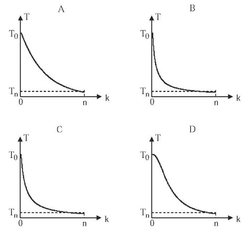
• Exponential multiplicative cooling (Figure 1-A), proposed by Kirkpatrick, Gelatt and Vecchi (1983), and used as reference in the comparison among the different cooling criteria. The temperature decrease is made multiplying the initial temperature T0 by a factor that decreases exponentially with respect to temperature cycle k:
• Logarithmical multiplicative cooling (figure 1-B), based on the asymptotical convergence condition of simulated annealing (Aarts, E.H.L. & Korst, J., 1989), but incorporating a factor a of cooling speeding-up that makes possible its use in practice. The temperature decrease is made multiplying the initial temperature T0 by a factor that decreases in inverse proportion to the natural logarithm of temperature cycle k:
• Linear multiplicative cooling (Figure 1-C). The temperature decrease is made multiplying the initial temperature T0 by a factor that decreases in inverse proportion to the temperature cycle k:
• Quadratic multiplicative cooling (Figure 1-D). The temperature decrease is made multiplying the initial temperature T0 by a factor that decreases in inverse proportion to the square of temperature cycle k:
Additive Monotonic Cooling
In the additive monotonic cooling, we must take into account two additional parameters: the number n of cooling cycles, and the final temperature Tn of the system. In this type of cooling, the system temperature T at cycle k is computed adding to the final temperature Tn a term that decreases with respect to cycle k. Four variants based on the formulae proposed by B. T. Luke (2005) are considered:
Figure 1. Multiplicative cooling curves: (A) Exponential, (B) logarithmical, (C) linear, (D) quadratic
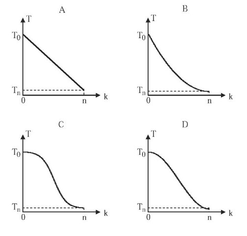
• Linear additive cooling (Figure 2-A). The temperature decrease is computed adding to the final temperature Tn a term that decreases linearly with respect to temperature cycle k:
• Quadratic additive cooling (Figure 2-B). The temperature decrease is computed adding to the final temperature Tn a term that decreases in proportion to the square of temperature cycle k:
• Exponential additive cooling (Figure 2-C). The temperature decrease is computed adding to the final temperature Tn a term that decreases in inverse proportion to the e number raised to the power of temperature cycle k:
• Trigonometric additive cooling (Figure 2-D). The temperature decrease is computed adding to the final temperature Tn a term that decreases in proportion to the cosine of temperature cycle k:
Non-Monotonic Adaptive Cooling
In the non-monotonic adaptive cooling, the system temperature T at each state transition is computed multiplying the temperature value Tk, obtained by any of the former criteria, by an adaptive factor m based on the difference between the current solution objective,
Figure 2: Additive cooling curves: (A) linear, (B) quadratic, (C) exponential, (D) trigonometric.
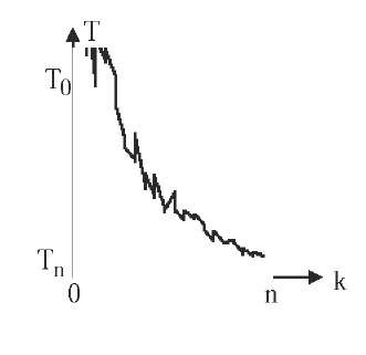
Figure 3. Curve of non-monotonic adaptive cooling
f(si), and the best objective achieved until that moment by the algorithm, noted f*:
Note that the inequality 1 < m < 2 is verified. This factor m means that the greater the distance between current solution and best achieved solution is, the greater the temperature is, and consequently the allowed energy hops. This criterion is a variant of the one proposed by M. Locatelli (2000), and it can be used in combination with any of the former criteria to compute Tk. In the comparison, the standard exponential multiplicative cooling has been used for this purpose. So the cooling curve is characterized by a fluctuant random behaviour comprised between the exponential curve defined by Tk and its double value 2Tk (Figure 3).
Combinatorial Optimization Problems Used in the Comparison
Travelling Salesman Problem. The Travelling Salesman Problem, TSP, consists of finding the shortest cyclic path to travel round n cities so that each city is visited only once. The objective function fto minimize is given by the expression:
where each variable xi means the city that is visited at position i of the tour, and d(xi,xj) is the distance between the cities xi and x.. The tests have been made using two different instances of the euclidean TSP. The first one obtains a tour of 47 European cities and the second one a tour of 80 cities.
Quadratic Assignment Problem. The Quadratic Assignment Problem, QAP, consists of finding the optimal location of n workshops in p available places (p > n), considering that between each two shops a specific amount of goods must be transported with a cost per unit that is different depending on where the shops are. The objective is minimizing the total cost of goods transport among the workshops. The objective function fto minimize is given by the expression:
where each variable xi means the place in which workshop i is located, c(xi,xJ) is the cost per unit of goods transport between the places where shops i and j are, and q(i,j) is the amount of goods that must be transported between these shops. The tests have been made using two different instances of the QAP: The first one with 47 workshops to be located in 47 European cities, and the second one with 80 workshops to be located in 80 cities.
Selection of parameters
For each problem instance, all variants of the algorithm use the same values of initial temperature T0 and number L of state transitions for each temperature. The initial temperature T0 must be high enough to accept any state transition to a worse solution. The number L of state transitions must guarantee with a probability n close to 1 that, if no solution changes are accepted, any k-neighbour solution near to the current one could be process.
In order to determine the other temperature decrease parameters of each cooling schedule under similar conditions of execution time, we consider the mean final temperature T and the temperature standard error c of the exponential multiplicative cooling of Kirkpatrick, Gelatt and Vecchi with decreasing factor a = 0.95. The objective is to determine the temperature decrease parameters in such a way that a temperature in the interval |T -c,T + c] is reached in the same number of cycles as the exponential multiplicative cooling. We distinguish three cases:
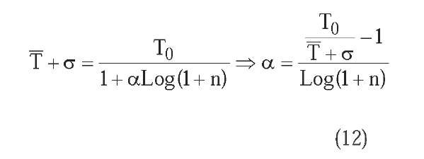
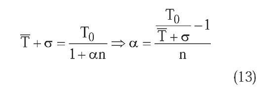
• Multiplicative monotonic cooling. The decrease factor a that appears in the temperature decrease equations must allow to reach the temperature T + ct , or highest temperature from which the end of the algorithm is very probable, in the same number n of cycles as the exponential multiplicative cooling. Knowing that for this cooling the number n of cycles is:
it results for the logarithmic multiplicative cooling:
for the linear multiplicative cooling:
and for the quadratic multiplicative cooling:
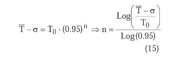
• Additive monotonic cooling. Final temperature is Tn = T – ct , and number n of temperature cycles is equal to the corresponding number of cycles of the exponential multiplicative cooling for that final temperature, that is:
• Non-monotonic adaptive cooling. As the adaptive cooling is combined in the tests with the exponential multiplicative cooling, the decrease factor a that appears in the temperature decrease equation must be also a = 0.95.
Analysis of Results
Table 1 shows the cooling parameters used on each instance of the TSP and QAP problems.
For each instance of the problems 100 runs have been made with the nine cooling schedules, computing minimum, maximum and average values, and standard error both of the objective function and of the number of iterations. For limited space reasons we only provide results for the QAP 80-workshops instance (Table 2). Local search results are also included as reference.
Considering both obj ective quality and number of iterations, we can conclude that the best cooling schedule we have studied is the non-monotonic adaptive cooling schedule based on the one proposed by M. Locatelli (2000), although without significant differences with respect to the exponential multiplicative and quadratic multiplicative cooling schedules.
FUTURE TRENDS
Complying with the former results we propose some research continuation lines on simulated annealing cooling schedules:
• Analyse the influence of the initial temperature in the performance of the algorithm. An interesting idea could be valuing the algorithm behaviour when the temperature is initialized with a percentage between 10% and 90% of the usual estimated value for T0.
• Determine an optimal monotonic temperature decrease curve, based on the exponential multiplicative cooling. A possibility could be changing the parameter a dynamically in the temperature decrease equation, with lower initial values (a = 0.8) and final values closer to 1 (a = 0.9), but achieving an average number of temperature cycles equal to the standard case with constant parameter a = 0.95.
• Study new non-monotonic temperature decrease methods, combined with the exponential multiplicative cooling. These methods could be based, as the Locatelli’s one in the comparison, on modifying the temperature according to the distance from the current objective to a reference best objective.
Table 1. Parameters of the cooling schedules
| TSP 47
T0 = 18000 L = 3384 |
TSP 80
T0 =110000 L = 9720 |
QAP 47
T0 = 3000000 L = 3384 |
QAP 80
T0 = 25000000 L = 9720 |
|
| Exp M SA | a = 0.95 | a = 0.95 | a = 0.95 | a = 0.95 |
| Log M SA | a = 267.24 | a = 2307.6 | a = 657.19 | a = 1576.64 |
| Lin M SA | a = 9.45 | a = 65.76 | a = 21.08 | a = 46.37 |
| Qua M SA | a = 0.0675 | a = 0.3593 | a = 0.13344 | a = 0.2635 |
| Additive SA | n = 156 Tn = 6.06 | n = 209 Tn = 2.46 | n = 181
Tn = 276.5 |
n = 197 Tn =1023 |
| Adapt SA | a = 0.95 | a = 0.95 | a = 0.95 | a = 0.95 |
Table 2. Results for QAP 80
| Min | Max | Average | Std. Error | ||
| LS | Objective | 251313664 | 254639411 | 252752757.8 | 716436.9 |
| Iterations | 27521 | 81118 | 46850.9 | 12458.1 | |
| Exp M SA | Objective | 249876139 | 251490352 | 250525795.8 | 344195.3 |
| Iterations | 684213 | 2047970 | 1791246.1 | 170293.2 | |
| Log M SA | Objective | 250455151 | 253575468 | 251745332.1 | 666407.2 |
| Iterations | 120248 | 2023073 | 696470.2 | 394540.2 | |
| Lin M SA | Objective | 249896097 | 251907025 | 250635912.2 | 391761.6 |
| Iterations | 653162 | 2250714 | 1428446.1 | 324475.7 | |
| Qua M SA | Objective | 249847174 | 251611701 | 250470415.8 | 350861.7 |
| Iterations | 1075019 | 2614896 | 1655619.1 | 294039 | |
| Lin A SA | Objective | 250641396 | 253763581 | 251874846.8 | 591713.9 |
| Iterations | 1946664 | 2552978 | 2008897.2 | 79027.1 | |
| Qua A SA | Objective | 250033262 | 251800841 | 250780492.4 | 391747.2 |
| Iterations | 1909770 | 2474159 | 1974620 | 89007.6 | |
| Exp A SA | Objective | 249833632 | 251808711 | 250665143 | 379160.5 |
| Iterations | 1799372 | 2939097 | 2080203.9 | 222456.5 | |
| Trig A SA | Objective | 250053171 | 252148088 | 250908285.3 | 431834.7 |
| Iterations | 1919964 | 2458885 | 1974441.2 | 77503.3 | |
| Adapt SA | Objective | 249902310 | 251553959 | 250481008.4 | 361964.3 |
| Iterations | 1564222 | 2455305 | 1803218.6 | 129649.9 | |
Although these three lines of work are independent, it seems to be clear that the ultimate objective would be integrating the results achieved with these lines, in order to build a high quality combinatorial optimization metaheuristic based on simulated annealing.
CONCLUSION
The main conclusions that can be drawn from the comparison among the cooling schedules of the simulated annealing algorithm are:
• Considering objective quality related to the shape of the temperature decrease curve, we can affirm that simulated annealing works properly with respect to the ability of escape from local minima when the curve has a moderate slope at the initial and central parts of the processing, and softer at the final part of it, just as it occurs in the standard exponential multiplicative cooling. The specific shape (convex, sigmoid) of the curve in the initial and central parts does not seem outstanding.
• Considering execution time, the standard error of the number of iterations seems to be related to the temperature decrease curve tail at the final part of the algorithm. An inversely logarithmic tail produces a softer final temperature fall and a higher standard error, while inversely quadratic and exponential tails cancel out faster, providing the best standard error values of the algorithm.
• Considering the use of a non-monotonic temperature decrease method, we can affirm that not only the utilized criterion does not make worse the general performance of the algorithm but it seems to have a favourable effect that deserves to be taken into account and studied in greater depth.
KEY TERMS
Combinatorial Optimization: Area of the optimization theory whose main aim is the analysis and the algorithmic solving of constrained optimization problems with discrete variables.
Cooling Schedule: Temperature control method in the simulated annealing algorithm. It must specify the initial temperature T0, the finite sequence of decreasing values of temperature, and the finite number L of state transitions for each temperature value.
Genetic and Evolutionary Algorithms: Genetic Algorithms (GAs) are approximate optimization algorithms inspired on genetics and the evolution theory. The search space of solutions is seen as a set of organisms grouped into populations that evolve in time by means of two basic techniques: crossover and mutation. Evolutionary Algorithms (EAs) are especial genetic algorithms that only use mutation as organism generation technique.
Local Search: Local search (LS) is a metaheuristic or general class of approximate optimization algorithms, based on the deterministic heuristic search technique called hill-climbing.
MemeticAlgorithms: MemeticAlgorithms (MAs) are optimization techniques based on the synergistic combination of ideas taken from other two metaheuris-tics: genetic algorithms and local search.
Simulated Annealing: Simulated Annealing (SA) is a variant of the metaheuristic of local search that incorporates a stochastic criterion of acceptance of worse quality solutions, in order to prevent the algorithm from being prematurely trapped in local optima.
Taboo Search: Taboo Search (TS) is a metaheuristic superimposed on another heuristic (usually local search or simulated annealing) whose aim is to avoid search cycles by forbidding or penalizing moves which take the solution to points previously visited in the solution space.


