Fast Evaluation of Appointment Schedules for Outpatients in Health Care (Queueing Theory) (Analytical and Stochastic Modeling) Part 2

Assisted Sequential Scheduling

Cost Function

The ‘quality’ of a schedule depends on the importance attributed to certain aspects of its performance. For example, it is a usual goal to keep the expected patient waiting times as low as possible, but not at the expense of an excessive physician idle time or session overtime. In most situations, to have the physician standing idle for 1 minute is deemed far less desirable than to keep a patient waiting for the same time period. In general, such differences in appreciation can be represented as a function of the performance criteria we have obtained in Section 2. For example, a suitable ‘cost’ function C associated with a particular schedule might be

where W and I respectively are

Thus formalised, the ‘best’ or optimal schedule is that which minimises the cost C. Other criteria such as the number of patients K, the physician lateness 0 or variances of waiting and idle times can also be taken into account, as well as specific costs related to particular (types of) patients. Clearly, the results obtained by optimalisation studies highly depends on what criteria are effectively considered in (17). For example, C depends only on W and I in [3,17,20,13], on W and the mean effective session duration tk+E[Wk] in [22,12], and on W, I, E[X] in [6,14].

Sequential vs. Advance Scheduling

As mentioned earlier, in appointment scheduling for outpatients, two methods can be distinguished. The first method is to fix the appointment immediately when the patient first calls in. This is called sequential scheduling [18,7], because the appointments are fixed one after the other, as the patients call in. Let t(k) and S(k) be the appointment time and consultation time of the kth calling patient respectively. If the schedule is already fixed for k patients, the decision at which time t(k +1) to schedule the next calling patient must then be based on the schedule so far, as well as on the distribution of S(k +1). Possibly, some global prospect of the future calling patients can be taken into account as well, in case such information is available or can be estimated. The most straightforward manner of sequential scheduling is to put the first calling patient at the start of the session, the next a short time later, and so on, until the end of the session is reached. This results in

and therefore t(k) = Tk. This is called First-come-first-appointment (FCFA) in [20]. However, one can also decide not to maintain the calling order in the schedule, i.e. t(k) = Tk, and put a new patient before a previously scheduled patient. This can be due e.g. to preference of the involved patient or because of other imposed time constraints. In any case, the problem with scheduling sequentially is that once a patient is assigned an appointment time it cannot be altered afterwards. If in hindsight it turns out that some minor adjustments would result in lower expected cost C, it is impossible to implement this.

This problem can be overcome by using a two-step procedure. First the desk administrator takes in the calls from all patients, without yet giving them an exact appointment time t(k). After enough (say K) patients have called for an appointment, the optimal schedule is determined, either by hand or by means of an automated search algorithm. Once the schedule is decided, each patient is contacted again and notified its appointment time Tk in the session. This method is referred to as advance scheduling, and will usually lead to a better schedule and lower cost C because it is optimised over all decision variables simultaneously, using the best available information on the consultation times of the involved patients. Formally, given K and tmax the optimalisation amounts to a nonlinear integer programming problem with decision variables 0 and t (k), k = 1,…,K in the range [0, tmax]. The objective is to determine the integer values that minimise the function (17) and are possibly subjected to some further constraints, e.g. on the range of Tk imposed by the patient or on the range of 0 by the physician. Note that although the decision space is finite, it may be extremely large. For example, assuming that 0 = 0 and A =1 minute, an exhaustive search to the optimal schedule for 20 patients on a 4 hour session still requires 24120 = 4.3• 1047 schedule evaluations. Even in case the order is irrelevant and (18) can be maintained, for example if all patients have the same consultation time distribution, the number of schedules is still (2260°) =3.8 • 1029. Another disadvantage of advance scheduling is clearly the additional administrative effort of having to contact patients twice.

Visualisation of Mean Performance

For now we restrict ourselves to the case of sequential scheduling and see how this process can be assisted as much as possible. Suppose a schedule for a particular session already exists when a new patient calls in. This patient must be added to the schedule by the administration in one of the tmax +1 slots. In doing so it would be useful to know, for each slot, the waiting time that the patient will experience if it were to be scheduled in that slot, as well as the incurred idle time for the physician. This information can be obtained from the schedule so far as follows, assuming 0 = 0 for clarity of reasoning.

Consider again the schedule as defined in the previous section, but disregard patients k+1 to K. That is, consider only the consultations of the first k patients with appointment times t1 to Tk. Let Rkii, 0 ^ i ^ tmax-Tk, denote the remaining work for the physician i slots after Tk, the last patient’s appointment. Likewise, define Jkii as the time that the physician has been idle in that slot. We refer to this quantity as the running idle time. With the auxiliary variable

we have

analogous to (4)-(5). Clearly, Rki and Jkii respectively correspond to the waiting time and idle time of an additional patient if it were to be scheduled in slot Tk+i, which is precisely the reason why these quantities are useful in sequential scheduling. Their moments can be calculated in exactly the same way as in (8)-( 11) and (14)-(16). We thus find

and

with

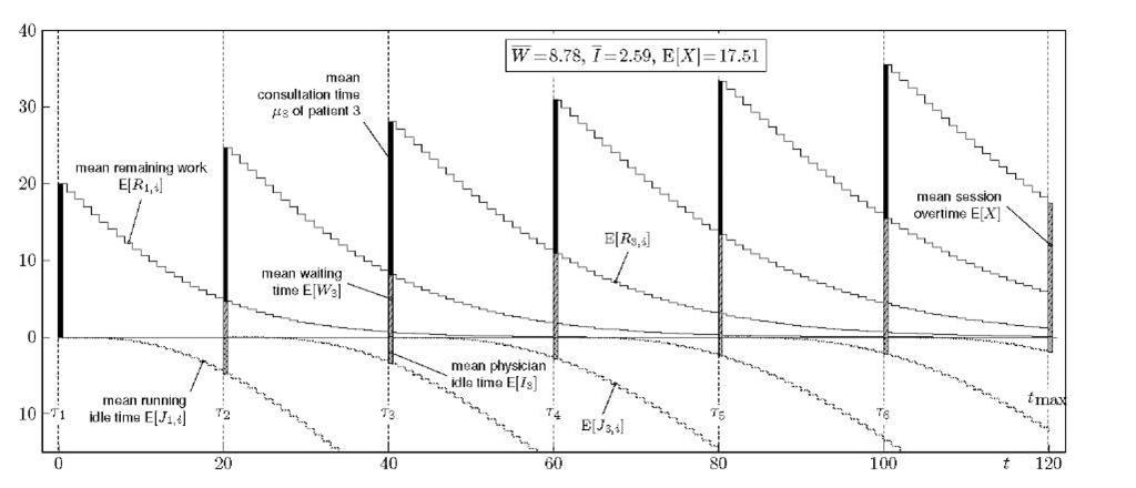
For example, the expected remaining work and running idle time for a session of length tmax = 120 with 6 already scheduled patients is visualised in Fig. 4. This graph shows the session on the horizontal axis and where the 6 patients are scheduled. For each patient k, E[Wk] and E[Ik] are plotted as a bar on the positive and negative vertical axis respectively, which shows the same information as in Figs. 1-3. Additionally, the black bar shows the mean consultation time which is the average workload each patient poses on the system. The graph also gives an idea of how the schedule performs in between appointments by showing the curves of the mean remaining work and running idle time. That is, for each slot t ^ Tk we show the average amount of time E[Rk,t-Tk] that the physician still has to spend in slot t on the first k patients. Likewise, the curves on the negative vertical axis show the average amount of time E[Jk,t-Tk] since the physician completed the consultation of patient k. Clearly, as the session progresses, the remaining work decreases while the running idle time increases. Note also that the remaining work due to the first k patients at the appointment time of the following patient coincides with that patient’s waiting time and likewise for idle times, i.e.

at least ifThis follows directly from the fact that (19)-(20) coincides with (4)-(5) for i = ak. In the same way, for i = 0 in (19)-(20) we have which, after taking expected values, is also evident from the graph.

Fig. 4. Visualisation of a schedule with tmax = 120 slots, 6 = 0 and K = 6 equidistant patients. For each patient k the mean remaining workis plotted and, in the negative vertical axis, the mean running idle timeThe mean consultation, waiting and idle time of each patient is also shown, as well as the expected overtime E[A'] at the end of the session. All patients have the same _T(20,150) consultation time distribution. For this session, we have

Although shown in Fig. 4 for demonstration purposes, it is not necessary to calculate E[Rk i] of the kth patient forthat is, beyond the appointment time of the next patient. Let us define the envelope of the mean remaining work curves and running idle time curves respectively as the functions

with

In the examples of Figs. 5 and 6 discussed below, the curves R(t) and J(t) on positive and negative vertical axis will be shown with a solid and dotted line respectively. Such a visual representation of the schedule’s average performance can assist the administrator if a new patient needs an appointment. For each slot t, the administrator can immediately see what the mean waiting and idle time for the new patient will be if it is appointed to that slot. If the new patient is effectively appointed to some slot t, everything from slot t onwards must be recalculated in order to visualise the new situation.

Examples

Let us consider a scenario where the patients are heterogeneous and have consultation times according to either of the four following distributions: (a) uniform between 5 and 15 minutes, (b) Poisson with a mean of 15 minutes, (c) r(20, 200) and (d) geometric with a mean of 25 minutes.

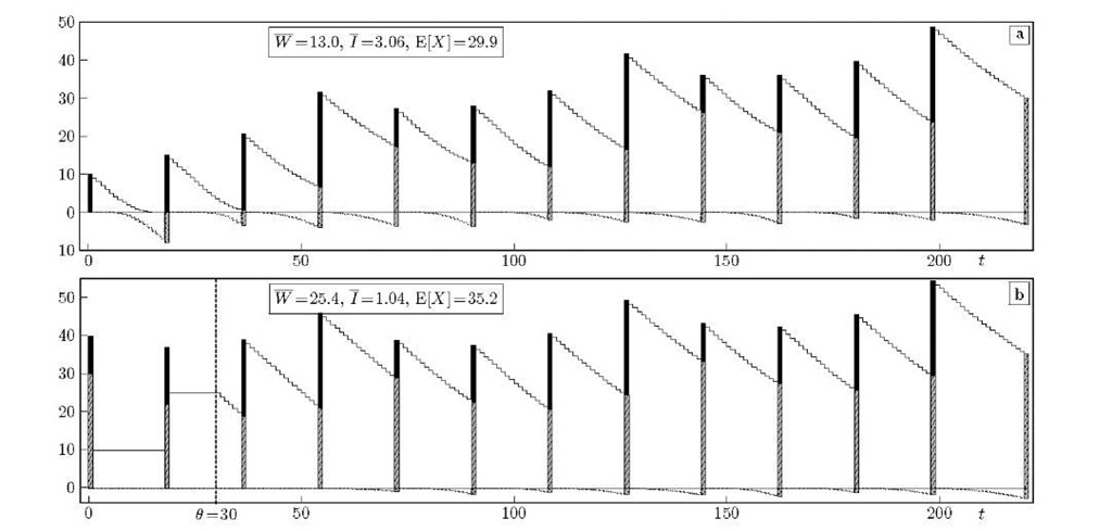
Fig. 5. Visualisation of a 4-hour session with 12 patients: remaining work R(t) and running idle time J(t) envelopes. The consultation times of the patients alternate between the four mentioned distributions. In (a), the patients are spaced at 18 minutes, which is about the overall mean of their consultation times. In (b) the physician arrives half an hour late.

These distributions have expected values 10, 15, 20, 25 and variances 10, 15, 200, 650 respectively. Let us assume that subsequent scheduled patients have consultation times circulating between these four distributions, i.e. S1 is distributed according to (a), S2 to (b), S3 to (c), S4 to (d), S5 to (a) again and so on. If it is not known to which type the consultation of a patient belongs to, we may assume that each type is equally likely which results in a pmfwith mean 17.5 and variance 250.

In Fig. 5 the visualisation of a 240-minute session is shown for K =12 patients. The administrator here does not take into account the heterogeneity of the patients and only uses the overall consultation time distribution as information. Patients are given appointments 18 minutes apart, which equals |~E[S]"|. So, even if for example the first patient cannot take more than 15 minutes, it is given an interval of 18 minutes. In (b) the same schedule is shown, but now the physician arrives 30 minutes after the start of the session. Although W increases considerably this way the mean idle time I is effectively reduced from 3.06 to 1.04 minutes. Note also that even though the physician starts 30 minutes later, the expected session overtime increased by only 5.3 minutes.

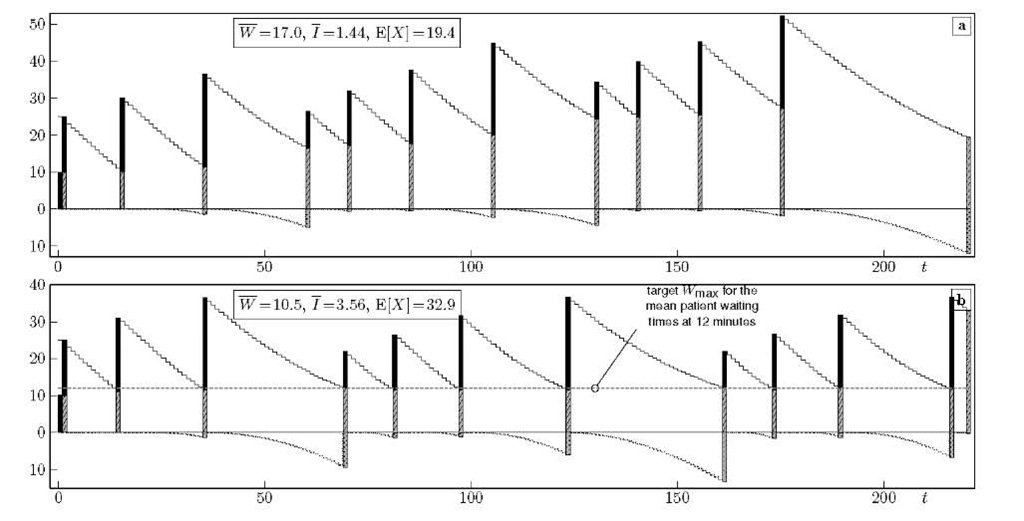
In Fig. 6 on the other hand, the administrator uses knowledge about the patient’s consultation type for scheduling. In (a) Bailey’s rule is applied: two patients are scheduled in the first slot while the rest are given an interval equal to their mean consultation time, we show an appointment rule that is particularly easy to apply if the envelopes R(t) and/or J(t) are available.

Fig. 6. Contrary to Fig. 5 the administrator knows which one of the 4 distributions each patient has. In (a) Bailey’s rule is followed, while in (b) all patients are targeted to have an expected waiting time of less than 12 minutes.

Suppose that our main optimalisation goal is fairness among patients, i.e. we want the mean waiting times E[Wk] to be more or less equal such that no patient is favoured by its position in the session. To achieve this, we can impose a target value Wmax for the mean patient waiting times of, say, 12 minutes which is indicated by the horizontal grey line. The point where this line intersects with the remaining work envelope R(t) is where the next patient will be scheduled. There is no sense in making the first patient wait however, which makes that W = 10.5 minutes instead of 12 minutes. This way of sequential scheduling could be extended by an additional target Imax for the idle times. If k patients are already scheduled, the appointment time of patient k +1 is decided by

with

Conclusions

We have proposed an analytic approach for evaluating appointment schedules on finite sessions that allows to obtain accurate results with very low computational complexity. By imposing a discrete-time setting and using Lindley’s recursion, we show that only a limited set W of waiting time probabilities need to be calculated in order to obtain the moments of waiting and idle times of the patients appointed to the session. The fact that the evaluation can be done very fast, makes our approach an ideal candidate for use in optimalisation studies. Additionally, we propose two new metrics that can assist in scheduling the patients sequentially: the mean remaining work and mean running idle time envelopes, which characterise the average performance of the schedule in each slot of the session.