Mathematical Preliminaries (Advanced Methods in Computer Graphics) Part 3

Curves

In Sect. 2.3, we came across the equation of a straight line expressed in terms of linear polynomials of a single parameter t (Eq. 2.12). Polynomials of a higher degree in t can be used to define curves in three-dimensional space. In the most general form, a curve can be represented as P(t) = (x(t), y(t), z(t)), where x(t), y(t), z(t) are continuous and differentiable functions of the parameter t. Polynomials of degree n have the property that their derivatives up to order n— 1 exist and are continuous over any finite interval in the parameter space. We can use the derivatives of the functions to define the tangential and normal directions to the curve at any point, and also to construct an orthonormal basis at any point on the curve.

The tangent vector at P(t) is given by the first derivative with respect to t, i.e., P’(t) = (x(t), y(t), z(t)). The unit tangent vector is denoted as

The tangent vector represents the local orientation of the curve at a point. If the parameter t denotes time, then P (t) represents the instantaneous velocity of the moving point P(t). The distance travelled from a starting point A = P(t0) to the current point, or in other words the arc length measured from A, is given by

Using the above equation we can express t as a function of arc length s, and re-parameterize the curve as P(s) = (x(s), y(s), z(s)). The chain rule for differentiation gives

from which we find that P’(s) is equivalent to the unit tangent vector T(t). For convenience, we denote P’(s) by T(s). Since T(s>T(s) = 1, it immediately follows that T(s>T’(s) = 0. Thus the instantaneous rate of change of the tangent direction is parallel to the normal vector at that point. If the unit normal direction at P(s) is denoted as N(s), we have

The proportionality factor k(s) is called the curvature of the curve at P(s). The curvature is a measure of the deviation of the curve from a straight line. For a straight line, k(s) = 0 at all points. The magnitude of the curvature is easily obtained as |k(s)| = T(s)|, and the unit normal direction at P(s) is given by

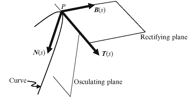
Fig. 2.8 Frenet frame attached to a curve at the point P

The plane containing the tangent vector and the normal vector is known as the osculating plane. The cross-product of the two unit vectors T(s) and N(s) gives the direction of the unit bi-normal vector denoted by B(s):

The three unit vectors T, N, B form an orthonormal basis as shown in Fig. 2.8. This local reference system is called the Frenet frame. The derivative of the binormal vector B’(s) is perpendicular to both B(s) and T(s), and hence parallel to N(s):

The term r (s) is called the torsion of the curve at s. Torsion is a measure of how much the curve deviates from the osculating plane.

The plane containing the tangent and binormal vectors is called the rectifying plane (Fig. 2.8). The plane formed by the normal and binormal vectors is called the normal plane.

The Frenet frame is useful for defining the local orientation of objects that move along a curved path. It can also be used for defining the eye-coordinate system for a camera that undergoes a curvilinear motion.

Affine Transformations

In this section, we consider linear transformations of three-dimensional points and vectors. The homogeneous coordinate system (Sect. 2.1) allows all transformations including translations to be represented using 4 x 4 matrices. We denote a translation by a vector v = (xv, yv, zv), by Tv, a rotation about the x-axis by an angle by 9, by Re(x), and a scaling by a vector k = (xk, yk, zk), by Sk (Box 2.3).

Box 2.3 Fundamental 3D Transformations (Fig. 2.9)

 

Fig. 2.9 Examples showing transformations of (a) a translation by an offset vector v (b) a rotation about the x-axis by an angle d and (c) scaling by factors kx, ky, kz

A linear transformation followed by a translation is called an affine transform. A general transformation can be given in matrix form as follows:

In the above equation, the matrix elements aij’s are all constants. (a03, ai3, a23) denote the translation components, and (xp, yp, zp, 1) the point on which the transformation is applied. The translation parameters do not have any effect on a vector (xv, yv, zv, 0). Under an affine transformation, line segments transform into line segments, and parallel lines transform into parallel lines. A fixed point of a transformation is a point that remains invariant under that transformation. For example, every point along the x-axis is a fixed point for the transformation R0(x). Similarly, the origin is a fixed point for the scale transformation. The most general rotation of an object with the origin as a fixed point, is the rotation by an angle 6 about an arbitrary vector v = (xv, yv, zv, 0) passing through the origin. The matrix for this transformation is given below.

where A = (1—cos0), B = sin0, and C = cos0. A rotation about an axis parallel to the x-axis, with an arbitrary fixed point P, can be obtained by first applying a translation T_p from P to the origin, a rotation R0 (x) with origin as the fixed point, and finally a translation Tp back to the original position P. In matrix form, we write the composite transformation as TpR0(x)Tp_1. Here T_1 denotes the inverse of the transformation T. For a translation, the inverse of Tp is T_p ; and for a rotation, the inverse of R0 (v) is R_0(v). A transformation of the form TRT-1 is called the conjugate of R.

We have just seen a few examples of affine transformations that are commonly used for generating new points by transforming existing ones. We could also combine the coordinates of a set of points using a linear equation to obtain a new point. Such interpolation methods are discussed in the next section.

Affine Combinations

A linear combination of a set of points Pi (i = 1,2,… n) produces a new point Q as shown below:

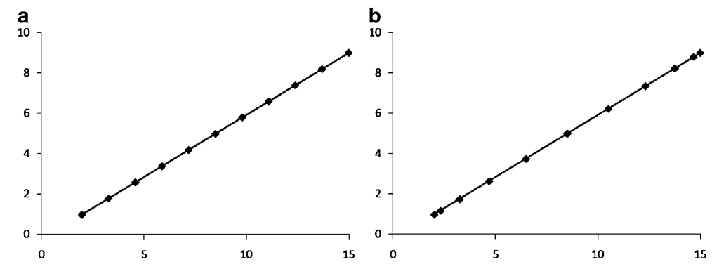
Fig. 2.10 (a) Linear interpolation and (b) trigonometric interpolation between two points where the coefficients (weights) wi are constants. If the weights satisfy the condition

then Eq. 2.41 gives an affine combination of points. Additionally, if wi > 0, for all i, then wi ’s form a partition of unity, and Eq. 2.41 is said to give a convex combination of points. As a special case, when n = 2, we get the formula for linear interpolation between two points Pi and P2:

An interesting variation of the above equation can be derived by expressing the parameter t as a function of an angle a, given by t = cos2a. Then the coefficient (1— t) becomes sin2a, and Eq. 2.43 takes the form Q = sin2a P1 + cos2a P2. However, this trigonometric interpolation formula gives a non-uniform distribution of points on the line when a is varied from 00 to 90° in equal steps. A comparison of linear and trigonometric interpolations is given in Fig. 2.10. In Fig. 2.10a, the parameter t is varied uniformly in the range [0-1] in steps of 0.1, and in Fig. 2.10b, the angle a is varied uniformly in the range [0-90] in steps of 91. Higher order interpolation between points is discussed in Chap. 7 (Box 2.4).

Box 2.4 Bernstein Polynomials

Given a positive integer value n, we can construct n + 1 polynomials of degree n of a parameter t as follows:

These polynomials form a partition of unity, i.e.,

Therefore, they can be used to generate convex combinations of points. Given n + 1 points Pi, i = 0,… ,n, we define a point Q(t) as

As the parameter t is varied from 0 to 1, we get a continuous parametric curve called the Bezier curve. The equations for n = 1, 2, 3 are given below.

First degree (linear): Q(t) = (1—t) Po + tP1

Second degree (quadratic) : Q(t) = (1—t)2P0 + 2(1—t)t P1 + t2P2

Third degree (cubic) : Q(t) = (1—t)3P0 + 3(1— t)21P1 + 3(1— t)tP + t3P3

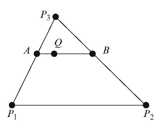
Fig. 2.11 A bilinear interpolation scheme first interpolates along the edges to get the values at A and B, and then uses another linear interpolation along the line AB to get the value at Q

Given a triangle with vertices P1, P2 and P3, we can perform a bilinear interpolation between the values defined at the vertices to get the interpolated value at an interior point Q (Fig. 2.11). Using this scheme, we can compute the colour value at any point inside a triangle, given the colour values at the vertices. A scan-line parallel to the base of the triangle sweeps the plane and generates the values of A and B using the linear interpolation equation in Eq. 2.43 with the same parameter t. Another linear interpolation between of A and B with a parameter s gives the value of Q. Thus we get

The above equation could be simplified into a simple convex combination of vertex points as

where k1 = s(1—t) and k2 = t. The bilinear interpolation of vertex coordinates shown above can be generalized to interpolate any quantity or attribute inside a triangle, given its values at the vertices. Examples of such vertex attributes are colour, texture coordinates and normal vectors. In the next section, we will consider another closely related interpolation method for triangles.