Geoscience Reference
In-Depth Information
100
-0.5
200
-1.5
1
-1
0.5
0.5
300
-0.5
400
500
600
700
800
-0.5
900
-0.5
60°N
40°N
20°N
Equator
20°S
40°S
60°S
Cooler surface
Warmer surface
Cooler surface
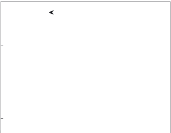
Figure 7.2. Annual mean, zonal mean meridional wind velocity (m/s; dark
gray contours) and vertical p-velocity (hPa/s; light gray contours). Shading
indicates downward motion. The contour interval for vertical velocity is
motion, and subsidence occurs over the cooler surfaces at subtropical latitudes
in both hemispheres.
Figure 7.2
provides a rudimentary view of the Hadley circulation, pieced
together by examining the zonal mean meridional and vertical velocity fields
jointly. A better way to envision and quantify the Hadley circulation is to de-
fine a stream function. Consider the three-dimensional velocity field in local
Cartesian
p
-coordinates, averaged around longitude,
t
t
v
|
[] [] [] [],
v ui vj
=++
ω
k
(7.1)
where the square brackets denote the zonal average. Because longitudinal (
x
-
coordinate) dependence is removed by taking the zonal mean,
[]/ 0
22
and
ux
the divergence of the zonal mean flow is
2
=+=
2
[]
[]
v
ω
v
d
$
[]
v
0
.
(7.2)
2
y
2
p
According to Eq. 7.2, convergence in the meridional direction must be bal-
anced by vertical divergence. In other words, only one independent variable,
either [
v
] or [], is needed to define the zonally averaged flow field. With a
little mathematical manipulation, a stream function, , can be used as that one
variable.
A simple way to define the stream function is with the following pair of
equations: