Geoscience Reference
In-Depth Information
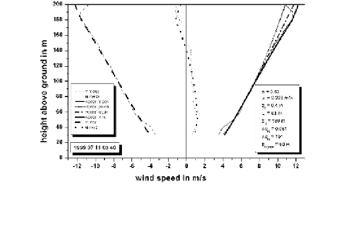
Fig. 3.18 Measured (thin full lines) and modelled (dotted from (
3.22
), dash-dotted (
3.16
), bold
(
3.80
)) vertical profiles of wind speed and its horizontal components u and v (modelled only) for
a rural area. Parameters for (
3.16
), (
3.22
) and (
3.80
) have been chosen in order to have coinciding
winds at 50 and 100 m, and are given in the right box. z
ref
= 50 m
with the following two examples from SODAR measurements over rural and
urban areas.
Figure
3.18
shows examples for vertical profiles of the west-east wind compo-
nent u and the south-north wind component v over flat terrain (z
0
= 0.1 m), Fig.
3.19
for an urban area (z
0
= 1 m). Both Figures demonstrate the ability of (
3.92
) and
(
3.93
) to describe the vertical turning of the wind underneath a low-level jet.
3.5 Internal Boundary Layers
The boundary layer flow structure over a homogeneous surface tends to be in
equilibrium with the surface properties underneath, which govern the vertical
turbulent momentum, heat, and moisture fluxes. When the flow transits from one
surface type to another with different surface properties, the flow structure has to
adapt to the new surface characteristics. This leads to the formation of an internal
boundary layer (IBL, internal because it is a process taking place within an
existing boundary layer) that grows with the distance from the transition line
(Fig.
3.20
).
An IBL with a changed dynamical structure can develop when the flow enters
an area with a different roughness (e.g. from pasture to forests or from agricultural
areas to urban areas) or crosses a coastline. An IBL with a modified thermal
structure can come into existence when the flow enters an area with a different
surface temperature (e.g. from land to sea or from water to ice). Often dynamical
and thermal changes occur simultaneously. Vertical profiles of wind, turbulence,
Search WWH ::

Custom Search