Geoscience Reference
In-Depth Information
equations for perhaps tens to hundreds of years of
simulated time depending on the question at
hand. In order to solve these coupled equations,
additional processes such as radiative transfer
through the atmosphere with diurnal and seasonal
cycles, surface friction and energy transfers and
cloud formation and precipitation processes must
be accounted for. These are coupled in the manner
shown schematically in
Figure 8.1
. Beginning with
a set of initial atmospheric conditions usually
derived from observations, the equations are
integrated forward in time repeatedly using time
steps of several minutes to tens of minutes at a
large number of grid points over the earth and at
many levels vertically in the atmosphere; typically
10-20 levels in the vertical is common. The
horizontal grid is usually of the order of several
degrees latitude by several degrees longitude near
the equator. Another, computationally faster,
approach is to represent the horizontal fields by a
series of two-dimensional sine and cosine
functions (a spectral model). A truncation level
describes the number of two-dimensional waves
that are included. The truncation procedure may
be rhomboidal (
R
) or triangular (
T
);
R
15 (or
T
21)
corresponds approximately to a 5° grid spacing,
R
30 (
T
42) to a 2.5
grid.
Realistic coastlines and mountains as well as
essential elements of the surface vegetation
(albedo, roughness) and soil (moisture content)
are typically incorporated into the GCM. These
are smoothed to be representative of the average
state of an entire grid cell and therefore much
regional detail is lost. Sea ice extent and sea surface
temperatures have often been specified by a
climatological average for each month in the past.
However, in recognition that the climate system
is quite interactive, the newest generation of
models includes some representation of an ocean
which can react to changes in the atmosphere
above. Ocean models (
Figure 8.2
) include a
so-called swamp ocean where sea surface temper-
atures are calculated through an energy budget
and no annual cycle is possible; a slab or mixed
layer ocean, where storage and release of energy
can take place seasonally and the most complex
°
grid, and
T
102 to a 1
°
SOLAR RADIATION
WATER BUDGET
MOMENTUM
BUDGET
O
3
CO
2
H
2
O CLOUDS
CONDENSATION
CONVECTION
EVAPORATION
TURBULENT
TRANSPORT
HEAT
BUDGET
INFRARED
RADIATION
HEAT DIFFUSION
PRECIPITATION
ICE
SNOW
EVAPORATION
ICE
FRICTION
MTN
(GROUND HEAT BUDGET)
TEMPERATURE
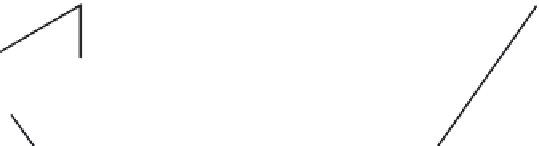
Figure 8.1
Schematic diagram of the interactions among physical processes in a general circulation model.
Source: From Druyan et al. (1975).