Geoscience Reference
In-Depth Information
hamburg
hamburg
breman
breman
byern
hesse
berlin
hesse
bwutt
bwutt
schleswi
byern
berlin
nrw
nrw
lowsax
rheinpa
rheinpa
schleswi
lowsax
brand
rheinpa
sax
sax-anh
.39
.41 .42
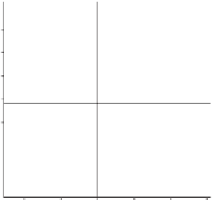
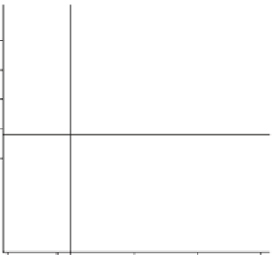
Inequality: Gini Market Income
.4
.43
.44
4
.45 .5 .55
Inequality: Gini Market Income
6
hamburg
hamburg
breman
breman
hesse
byern
bwutt
byern
berlin
hesse
bwutt
nrw
schleswi
nrw
berlin
lowsax
rheinpa
rheinpa
lowsax
schleswi
sax
brand
sax-anh
meekl
thur
.2
.22 .24 .26
Inequality: Gini Disposable Income
.28
.2
.22 .24 .26
Inequality: Gini Disposable Income
.28
.3
FIGURE 6.2. The Geography of Income Inequality before and after Reunification
inequality in both years.
8
A number of aspects of
Figures 6.1
and
6.2
are worth
noting.
Germany's level of gross state product (GSP) per capita was significantly
lower in 1993-1994 than it was in 1989, as reflected by the decrease over time
in the horizontal line depicting, in both figures, the l anders' average GDP per
capita. The incorporation of the eastern l ander contributed to a reduction of
the amount of resources per inhabitant available to the union. This develop-
ment relates in turn to a second aspect of the process captured by
Figure 6.1
:an
extreme gap in terms of the ability of different regional economies to generate
employment. Even as late as 1993, four years after the programs of economic
recovery for the East had begun, the East alone constituted a major factor
skewing the geography of unemployment. The range of variation among the
8
Figures represent Gini coefficients for household market and disposable income per equivalent
adult. These calculations were performed by the author on the basis of LIS data (1989, 1994;
full sample). The equivalent scale used is the standard square root of the number of members of
the household.