Doppler radar analysis techniques - Severe Convective Storms and Tornadoes: Observations and Dynamics - page 430

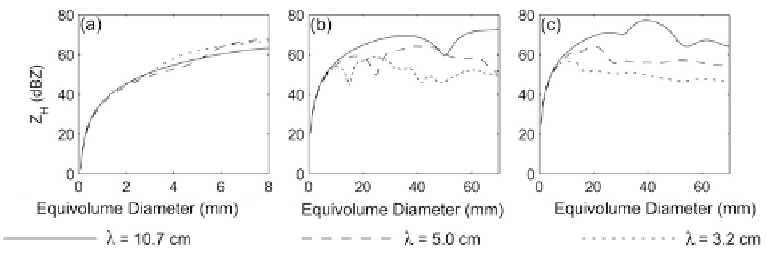
Figure A.4. Comparison of the variation of horizontally polarized radar reflectivity factor
(Z H ) for hydrometeor type and size at the S-band (solid line), C-band (long-dashed line),
and X-band (short-dashed line): (a) for rain; (b) for ''dry hail'' with 0% fractional water;
(c) for ''wet hail'' with 10% fractional liquid water content. Z H was calculated for rain at 10 C,
a mean canting angle and a canting angle standard deviation of 0 , and a liquid water content
of 10 gm 3 ; for dry hail with ice content of 2 gm 3 ,0 mean canting angle, and 60 canting
angle standard deviation; for wet hail with conditions the same as those for dry hail, but with a
canting angle standard deviation of 55.2 . Note how, for both dry and wet hail, the relationship
between Z H and size is not monotonic for equivolume diameters in excess of 10-15mm, well
into the Mie scattering range especially at the X and C-bands (from Snyder et al., 2010).

(A.2) for u and v . Vertical velocity w is then computed kinematically using a
lower-boundary condition (such as w ¼ 0atz ¼ 0) and then u and v are solved
again using (A.1) and (A.2), and so on until the solutions for u, v ,andw converge.
(It is also possible to impart an upper-boundary condition also, if data are avail-
able high enough up in the storm so that one can assume, for example, that w ¼ 0
at the top; if so, then an adjustment scheme is employed to redistribute the error
in horizontal divergence with height. Or, for airborne radars, one may integrate
downward.)
The variational method, pioneered by Yoshi Sasaki in the 1960s, makes use of
a cost function J, which is minimized. The cost function is arbitrary and may be
composed of a number of components, so that, for example

J ¼ J 1 þ J 2 þþ J n ð A : 5 Þ

The first cost function J 1 represents the square of the difference between
interpolated Doppler (radial) wind speeds and actual, measured Doppler wind
speeds at each radar at each gridpoint, weighted by the square of the distance
from the radar to account for beam spreading; the second cost function is the
square of the continuity equation set to zero, which acts as a ''weak'' continuity
constraint on the three-dimensional wind field (i.e., the wind field that minimizes
the residual left over in the least square sense when applying the continuity equa-
tion, so that the equation of continuity is not satisfied exactly; it is therefore
termed a ''weak'' constraint); other cost functions may also be used, such as the
square of the time-dependent vorticity equation set to zero, which acts as a weak