Tornadoes - Severe Convective Storms and Tornadoes: Observations and Dynamics - page 375

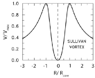
Figure 6.48. Radial (R) profile of azimuthal (tangential) wind (V) in a Sullivan vortex. R core is
the core radius; V max is the maximum azimuthal wind speed (adapted from Brown and Wood,
2012).

radial distribution of vertical velocity is given by

r Þ¼ 2az ½ 1 3 exp ð ar 2 w ð z ; = 2 Þ ð 6 : 41 Þ

So, unlike the Burgers-Rott vortex, vertical velocity is a function of both height
and radius. It can be seen that the azimuthal component of vorticity in a Sullivan
vortex is

¼ð JT v Þ ' ¼ 6a 2 rz exp ð ar 2

= = 2 Þ ð 6 : 42 Þ

which is greatest at

0 : 5

r ¼ð= a Þ ð 6 : 43 Þ

so that there is a circular ring of horizontal vorticity in the clockwise direction
associated with sinking motion at the center and rising motion at greater distance
from the center. Finding steady-state analytic solutions is an art and may be
pursued usefully up to a point, but it then becomes more worthwhile to integrate
the equations of motion numerically to find solutions. Because the Sullivan
vortex also includes vertical motions, it is the most realistic of the analytic vortex
solutions when there is surface friction.
While solutions for the behavior of boundary layers for solid-body rotation
and potential flow have been solved for separately, as noted earlier, it was not
until H. L. Kuo, in a mathematically complicated 1971 paper, described the solu-
tions to the problem for a Rankine combined vortex, for which motions in both
regimes are coupled to each other; for turbulent flow, Kuo used the boundary
condition

v ¼ Kdv = dz at z ¼ 0 ð 6 : 44 Þ

where K ¼ 0, for no-slip boundary conditions; and K

>

0 for some degree of
''slip''. He found that in the solid-body rotation region, inside the core, the