The deep interior of the Earth - The Solid Earth - page 339

(b)

% d V s / V s

--1.6 --1.2 --0.8 --0.4 0.0 +0.4 +0.8 +1.2 +1.6

-1.6 -1.4 -1.2 -1.0 -0.8 -0.6 -0.4 -0.2 0.0 0.2 0.4 0.6 0.8 1.0 1.2 1.4 1.6

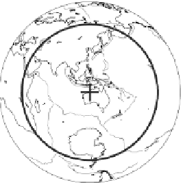
Figure 8.6. (b) The long-wavelength S-wave velocity-perturbation model viewed as
a slice through the centre of the Earth along the great circle shown as the blue circle
in the central map. Note the two extensive slow (red) anomalies beneath Africa and
the central Pacific that start at the CMB, the base of the lower mantle. Black circle,
boundary between upper and lower mantle at 670 km. Colour version Plate 10.(T.G.
Masters, personal communication 2003.
http://mahi.ucsd.edu/Gabi/rem2.dir/shear-models.htm.)

orange. At shallow depths in the upper mantle the mid-ocean-ridge system has
low Q while the continental regions have high Q .
Higher-resolution, global body-wave models of the mantle have until recently
been limited by (i) the quality of the short-period data and (ii) uncertainties
in earthquake locations. However, there have been significant advances and
−→

Figure 8.6. (c) A comparison of P- and S-wave velocity models for the lower mantle
at depths of 800, 1050, 1350, 1800, 2300 and 2750 km. The models are shown as
perturbations from a standard whole-Earth model. The P-wave model was
calculated using 7.3 million P and 300 000 pP travel times from ∼80 000 well-located
teleseismic earthquakes, which occurred between 1964 and 1995 (van der Hilst et al .
1997). The S-wave model used 8200 S, ScS, Ss, SSS and SSSS travel times (Grand
1994). The number at the side of each image indicates the maximum percentage
difference from the standard model for that image. White areas: insufficient data
sampling. Colour version Plate 11. (From Grand and van der Hilst, personal
communication 2002, after Grand et al .(1997).)