Geoscience Reference
In-Depth Information
RMS VELOCITY (km s
−
1
)
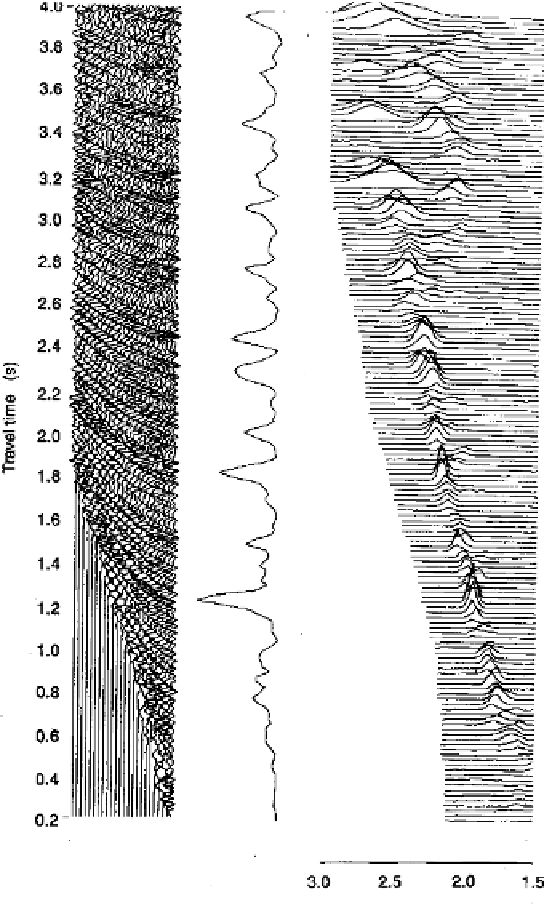
Figure 4.42.
Steps in the computation of a velocity analysis. (a) The twenty-four
individual reflection records used in the velocity analysis. (b) The maximum
amplitude of the stacked trace shown as a function of
t
0
, two-way time along the
trace. Notice that the reflections are enhanced compared with the original traces.
Although the main reflections at
t
0
= 1.2 and 1.8 s do stand out on the original
traces, these intercept times are clearly defined by the stacked trace, and
subsequent deeper reflections that were not clear on the original traces can now be
identified with some confidence on the stacked trace. (c) The velocity spectrum for
the traces in (a). The peak power at each time served to identify the velocity which
would best stack the data. The stacking velocity clearly increases steadily with depth
down to about 3 s. After this, some strong multiples (rays that have bounced twice
or more in the upper layers and therefore need a smaller stacking velocity) confuse
the velocity display. (From Taner and Koehler (1969).)