Geoscience Reference
In-Depth Information
The Wedge Model
−
0.2
0
0.2
−
0.2
0
0.2
−
0.2
0
0.2
0
0
0
20
40
60
80
100
120
140
160
20
20
40
40
60
60
Wedge Model
80
80
100
100
120
120
140
140
160
160
50
2
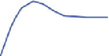
Tuning Curve
40
1.5
30
1
20
0.5
10
0
0
0
20
40
60
true thickness (ms)
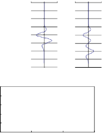
Fig. 4.2
Schematic wedge model for tuning effects.
noise, and the extent of complications from the presence of other adjacent layers. If it
is, say, half the resolution limit, this implies that the standard seismic method will see
only those layers whose thickness is greater than say 20 ft.
the amplitude response and apparent thickness of a sand bed encased in shale, using
a zero-phase wavelet, and increasing the bed thickness from zero through the tuning
range. As expected, there is a linear increase in amplitude with true thickness when
the bed is thin, while the apparent thickness remains constant. There is a maximum
amplitude produced by constructive interference, where the precursor of the reflection
from the base of the sand is added to the main lobe of the reflection from the top of
the sand. Beyond this point, the top and base of the sand are observable as separate
reflectors, and the amplitude falls to the value expected for an isolated top sand reflector.
Figure 4.3
shows an example on an actual seismic line. The amplitude of the gas sand
reflection is highest (bright yellow) on the flanks of the structure where there is tuning
between the top of the gas sand and the gas-water contact, and decreases towards the
crest of the structure (orange-red) where the gas column is greater; in this particular
example, the column is never great enough to resolve the gas-water contact as a separate
event. In map view, the result will be a doughnut-shaped amplitude anomaly, with the
highest amplitudes forming a ring around the crest at the point where the tuning effect
produces the highest amplitude.