MassFLOW-3DTM as a simulation tool for turbidity currents: some preliminary results - From Depositional Systems to Sedimentary Successions on the Norwegian Continental Margin - page 591

Body Neck Head

0.0

0.05

0.1 0

3.0 2.0

Colour bar [ms -1 ]

1.0

Time (s)

0 0.2 0.4 0.6 0.8 1 1.2

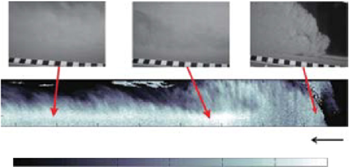
Fig. 2. Visual and velocity data of the passage of the head of the experimental turbidity current. (Top row) Three snapshots
of the current taken with a high speed camera. The top row consists of three camera images of the high-density turbidity
current. Black and white squares in the bottom of the image are 1 × 1 cm and the flow direction is from left to right. (Below)
The velocity data collected by the UVP.

Figs 4A and B show a comparison of the veloci-
ties in the head of the high-density turbidity cur-
rent in both the numerical and experimental
set-up. Fig. 4C shows the sediment concentration
for one of the performed simulations (Run 15 f in
Table 1A). During the experiments, the UVP probe
measured the velocities in the direction of the
probe (45° with respect to the flume floor) at 128
bins spread over the full depth of the flow. One
such cycle over 128 bins lasted for 14 ms. In order
to compare directly the experimental velocity val-
ues with the numerical ones, the latter ones had to
be calculated at the same angle as the UVP probes.
The simulated velocity magnitudes in the head of
the flow agree with the experimental results rather
well (Fig. 4). Both datasets indicate a rather uni-
form velocity profile in the nose of the current.
Furthermore, both datasets show that the maxi-
mum velocities occur in the back of the head
(neck) where the body of the turbidity currents
enters the head. Both simulations show that the
incoming flows are decelerated in the head and
start to detach from the bed. The shape and the
velocity values for the numerical simulations
match the observations from the laboratory. The
highly-turbulent environment is reproduced well
and the numerical parameters in the software only
slightly change the solution of the performed runs
(as shown in Fig. 3). This confirms the capability
of the software to model, in a realistic way, a
highly turbulent and transient environment at the
front and head of a turbidity current.

Case Study I-b: Body of the flow - mono
dispersed mixture

The body of the turbidity current follows the head
of the flow (Meiburg & Kneller, 2010). While the
head passes the control section in a limited time
period, the body continues flowing for an extended
time (approximately 1 minute in the experiments)
and it is influenced by the presence of suspended
and deposited sediments already in the system
due to the passage of the head of the flow itself.
Moreover, the body of the turbidity current expe-
riences fluctuations in both concentration and
velocity due to the instabilities on the interface
between the current and the ambient fluid
(Cartigny, 2012).
Time averaged velocity profiles were constructed
to smoothen these instabilities and facilitate a
comparison between the numerical and physical
datasets.
In the physical model, a steady state velocity pro-
file of the body of the high-density turbidity current
was calculated by averaging the velocity profiles
that were measured during the passing of the body
under the UVP (Fig. 5). Fig. 6A shows the velocity
profiles of the body of the turbidity currents for all
the runs reported in Table 1B, measured 2.6 m
from the inlet and averaged over a 53 s period, as
well as the UVP profile from the physical experi-
ment. In all the numerical simulations, the aver-
aged velocity profiles have a peak of about 1.1 m s −1
approximately 2 cm above the flume floor. Above