Geoscience Reference
In-Depth Information
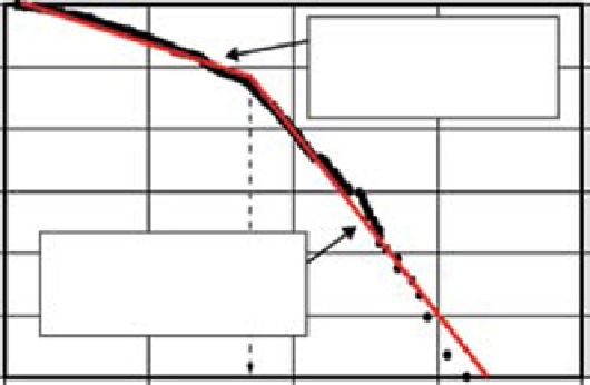
plot of the measured cross-set thicknesses, using
their logarithm values (log
x
) and logarithmic fre-
quency, log
EF
(
x
), appears to be best matched by a
lognormal distribution curve (Fig. 15), with a
goodness-of-fit slightly in excess of 98%. However,
the dataset distribution can be almost equally well
approximated by two straight regression lines,
each with a goodness-of-fit coefficient of ~ 98%
(Fig. 16). The same bipartition with a break-point
thickness value
x
b
≈ 43 cm characterises data
subsets from the individual wells, which implies a
homogeneous data population with a statistical
property that is stationary (i.e. laterally persistent).
A similar property of tidal dune cross-sets has
been recognised by Longhitano & Nemec (2005).
The linear trend means that the dataset can be
approximated by a two-tier power-law distribu-
tion and regarded as a bimodal fractal population
(Turcotte, 1992; Middleton
et al
., 1995). The
fractal dimension, estimated as the trend-line gra-
dient, is
D
1
= 0.78 for the thickness range of 7 cm to
43 cm and
D
2
= 2.78 for the thicker cross-sets in the
measured range of 43 cm to 250 cm (Fig. 16). The
minimum cross-set thickness has been taken as
x
min
= 7 cm, which is the minimum dune height
(Ashley, 1990). The maximum cross-set thickness
measured in cores is
x
max
= 250 cm, although an
extension of the lognormal curve to the lower fre-
quency limit (Fig. 15) suggests that one cannot
preclude possible rare cross-sets up to 840 cm thick,
not encountered in the studied cores.
The fractal approximation has important impli-
cations for the spatial heterogeneity of the sedi-
mentary succession (Stølum, 1991) and gives two
major advantages in the present case. Firstly, it
allows the frequency distribution of the cross-set
thicknesses in their two ranges to be described
fully by a single statistic, the fractal dimension
(
D
). The use of Gaussian statistics, such as an
arithmetic mean and standard deviation, would
be meaningless for the raw dataset, because its
frequency distribution is not normal. Second, it
allows the frequency distribution of cross-set vol-
umes to be estimated on the basis of Malinverno's
(1997) statistical theory.
Cross-set volume distribution
— The geometrical
relationships used here have been adopted from
Malinverno (1997) and are reviewed in the Appendix.
Although Malinverno's theory was originally used
for turbidite beds, it is by no means generic and
accounts for the geometry and spatial stacking pat-
tern of beds irrespective of their origin. Arguably,
some of the theory's assumptions are better suited
for dune cross-sets (Longhitano & Nemec, 2005) than
for lobate turbidite beds tapering with distance.
Malinverno (1997) derived a theoretical rela-
tionship between the frequency distribution of
bed thicknesses and the frequency distribution of
bed volumes, assuming that the former can be
approximated by a power-law distribution:
−
D
(5)
EF xx
i
()≈
i
0.000
1.000
Subpopulation 1
Cross-set thickness range: 7- 43 cm
n
= 501
R
2
= 0.979 (
SL
= 0.05%)
Fractal dimension
D
1
= 0.78
-0.500
0.316
0.100
-1.000
-1.500
0.031
Subpopulation 2
Cross-set thickness range: 43-250cm
n
= 165
R
2
= 0.984 (
SL
= 0.05%)
Fractal dimension
D
2
= 2.78
-2.000
0.010
-2.500
0.003
-3.000
0.800
0.001
log
x
b
=1.63
1.300
1.800
Cross-set thickness logarithm (log
x
)
2.300
2.800
Fig. 16.
The exceedence frequency distribution of measured dune cross-set thicknesses approximated as a two-tier power-
law distribution. Letter symbols:
n
− number of data in subpopulation;
R
2
− coefficient of determination (regression line
goodness of fit);
SL
= 0.05% is the significance level and means 99.95% confidence for the linear trend;
D
− subpopulation
fractal dimension (regression line gradient).
Search WWH ::

Custom Search