Dynamics and Electrodynamics of the Mesosphere - The Earth's Ionosphere: Plasma Physics and Electrodynamics - page 346

Meridional wind

90

z B

80

e z/2H

70

60
2 20 0 20 40 60 2 1 0 12 3 0 20 40 60

N 2 /N 0 Velocity (m/s) R i

(a) (b) (c)

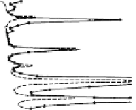
Figure 7.4 A comparison between height profiles of (a) meridional wind velocity,
(b) normalized total static stability

N 2 N 0 ) in the meso-

sphere (see Eq. (5.27)). The solid, dashed, and dot-dashed lines in the wind profile indicate
the measured meridional wind, the mean flow, and a hypothetical exponential growth
of the wind perturbation, respectively. [After Muraoka et al. (1988). Reproduced with
permission of the American Geophysical Union.]

( / and (c) Richardson number ( R i )

and the potential temperature is simply advected, u can be expressed in terms

of the wave-induced potential temperature perturbation

δ

(δθ)

by

i d

dz

θ/

δθ = δ u (7.2)

m ( c − u )

= √ − is 90 ◦ out of phase with where i represents the

background potential temperature profile, and m is the vertical wave number.
The Brunt-Väisälä frequency, N , can be related to

1 indicates that δθ δ u ,θ( z )

θ

by

N 2

= ( /θ)( θ/ )

g d dz (7.3)

Following atmospheric science tradition, we use N for the Brunt-Väisälä fre-
quency in this chapter rather than ω b . Recall that if N 2 is positive, a parcel of air

will oscillate at the radian frequency N if it is displaced vertically by a distance
of z from its equilibrium altitude, that is, the subsequent motion is described

by the real part of

δ

ze − iNt z ( t ) = δ (7.4)